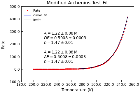
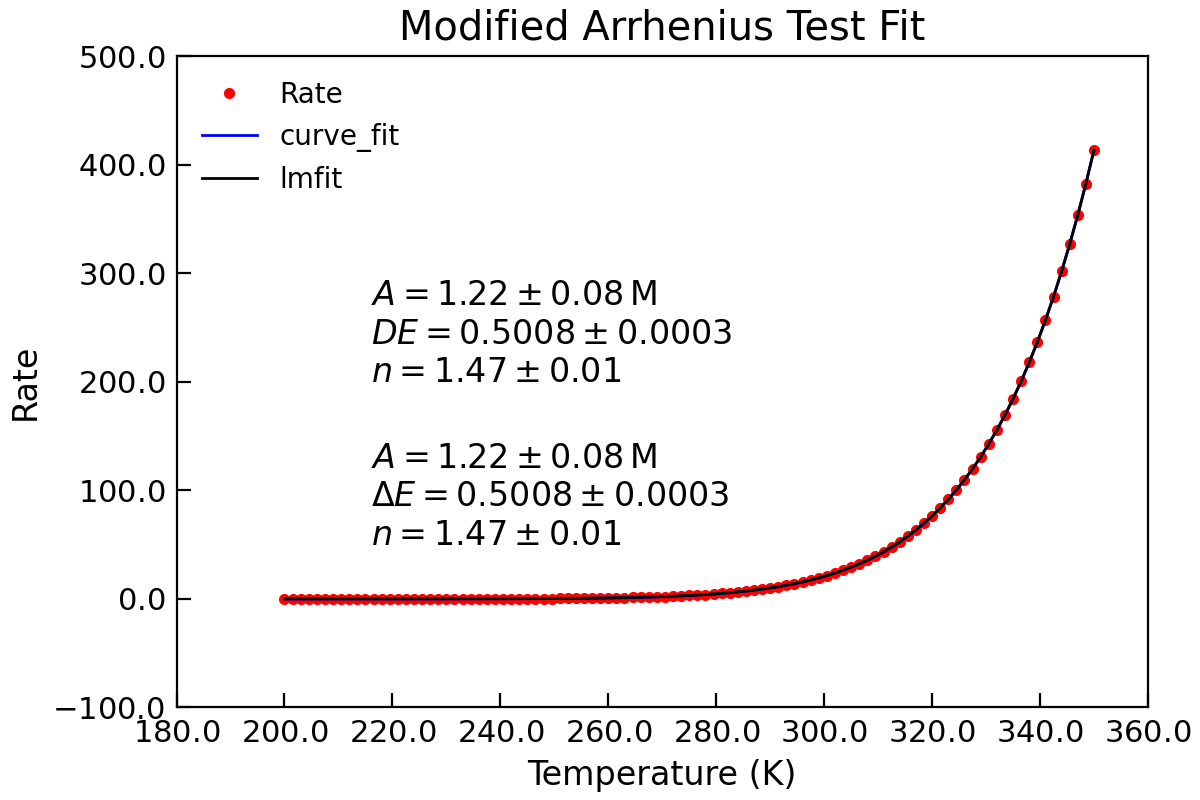
modArrhenius

Stoner.analysis.fitting.models.thermal.modArrhenius(x, A, DE, n)

Arrhenius Equation with a variable T power dependent prefactor.

Parameters:

• x (array) – temperatyre data in K

• A (float) – Prefactor - temperature independent. See :py:func:modArrhenius for temperaure dependent version.

• DE (float) – Energy barrier in eV.

• n (float) – The exponent of the temperature pre-factor of the model

Returns:

Typically a rate corresponding to the given temperature values.

The modified Arrhenius function is defined as \(\tau=Ax^n\exp\left(\frac{-\Delta E}{k_B x}\right)\) where \(k_B\) is Boltzmann’s constant.

Example

"""Example of nDimArrhenius Fit."""
from numpy import linspace
from numpy.random import normal

from Stoner import Data
from Stoner.analysis.fitting.models.thermal import modArrhenius, ModArrhenius

# Make some data
T = linspace(200, 350, 101)
R = modArrhenius(T, 1e6, 0.5, 1.5) * normal(scale=0.00005, loc=1.0, size=len(T))
d = Data(T, R, setas="xy", column_headers=["T", "Rate"])

# Curve_fit on its own
d.curve_fit(modArrhenius, p0=[1e6, 0.5, 1.5], result=True, header="curve_fit")
d.setas = "xyy"
d.plot(fmt=["r.", "b-"])
d.annotate_fit(modArrhenius, x=0.2, y=0.5, mode="eng")

# lmfit using lmfit guesses
fit = ModArrhenius()
p0 = [1e6, 0.5, 1.5]
d.lmfit(fit, result=True, header="lmfit")
d.setas = "x..y"
d.plot()
d.annotate_fit(ModArrhenius, x=0.2, y=0.25, prefix="ModArrhenius", mode="eng")

d.title = "Modified Arrhenius Test Fit"
d.ylabel = "Rate"
d.xlabel = "Temperature (K)"

(png, hires.png, pdf)