arrhenius

Stoner.analysis.fitting.models.thermal.arrhenius(x, A, DE)

Arrhenius Equation without T dependent prefactor.

Parameters:

• x (array) – temperatyre data in K

• A (float) – Prefactor - temperature independent. See :py:func:modArrhenius for temperaure dependent version.

• DE (float) – Energy barrier in eV.

Returns:

Typically a rate corresponding to the given temperature values.

The Arrhenius function is defined as \(\tau=A\exp\left(\frac{-\Delta E}{k_B x}\right)\) where \(k_B\) is Boltzmann’s constant.

Example

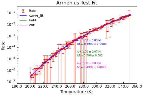
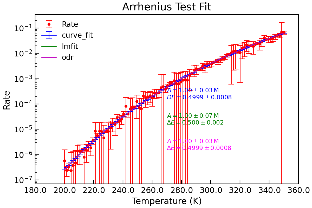
"""Example of Arrhenius Fit."""
from numpy import linspace, ceil, log10, abs as np_abs
from numpy.random import normal

from Stoner import Data
from Stoner.analysis.fitting.models.thermal import Arrhenius, arrhenius

# Make some data
T = linspace(200, 350, 101)
R = arrhenius(T + normal(size=len(T), scale=3.0, loc=0.0), 1e6, 0.5)
E = 10 ** ceil(log10(np_abs(R - arrhenius(T, 1e6, 0.5))))
d = Data(T, R, E, setas="xye", column_headers=["T", "Rate"])

# Curve_fit on its own
d.curve_fit(arrhenius, p0=(1e6, 0.5), result=True, header="curve_fit")
d.setas = "xyey"
d.plot(fmt=["r.", "b-"])
d.annotate_fit(
    arrhenius,
    x=0.5,
    y=0.5,
    mode="eng",
    fontdict={"size": "x-small", "color": "blue"},
)

# lmfit using lmfit guesses
fit = Arrhenius()
d.setas = "xye"
d.lmfit(fit, result=True, header="lmfit")
d.setas = "x...y"
d.plot(fmt="g-")
d.annotate_fit(
    Arrhenius,
    x=0.5,
    y=0.35,
    prefix="Arrhenius",
    mode="eng",
    fontdict={"size": "x-small", "color": "green"},
)

d.setas = "xye"
res = d.odr(Arrhenius, result=True, header="odr", prefix="ODR")
d.setas = "x....y"
d.plot(fmt="m-")
d.annotate_fit(
    Arrhenius,
    x=0.5,
    y=0.2,
    prefix="ODR",
    mode="eng",
    fontdict={"size": "x-small", "color": "magenta"},
)


d.title = "Arrhenius Test Fit"
d.ylabel = "Rate"
d.xlabel = "Temperature (K)"
d.yscale = "log"

(png, hires.png, pdf)