Cookbook
This section gives some short examples to give an idea of things that can be done with the Stoner python module in just a few lines.
The Util module
The Stoner package comes with an extra Stoner.analysis.utils module that includes some handy utility
functions.
The Data Class
The Stoner.Data class provides the core object for analysing data.
from Stoner.Core import Data d=Data(“File-of-data.txt”)
Splitting Data into rising and falling values
So far the module just contains one function that will take a single Stoner.Core.DataFile
object and split it into a series of Stoner.Core.DataFile objects where one column is either
rising or falling. This is designed to help deal with analysis problems involving hysteretic data.:
from Stoner.analysis.utils import split_up_down
folder=split_up_down(data,column)
In this example folder is a Stoner.DataFolder instance with two groups, one for rising values of the column
and one for falling values of the column. The split_up_down() will take an optional third parameter
which is an existing Stoner.Core.DataFolder instance to which the new groups (if they
don’t already exist) and files will be added.
Analysis of Hysteresis Loops
Since much of our group’s work is concerned with measuring magnetic hystersis loops, the hysteresis_correct() function
provides a handy way to correct some instrumental artifacts and measure properties of hysteresis loops.:
from Stoner.analysis.utils import hysteresis_correct
d=hysteresis_correct('QD-SQUID-VSM.dat',correct_background=False,correct_H=False)
e=hysteresis_correct(d)

print "Saturation Magnetisation = {}+/-{}".format(e["Ms"],e["Ms Error"])
print "Coercive Field = {}".format(e["Hc"])
print "Remanance = {}".format(e["Remenance"])
The keyword arguments provide options to turn on or off corrections to remove diamagnetic background (and offset in M), and any offset in H (e.g. due to trapped flux in the magnetometer). The latter option is slightly dangerous aas it will also remove the effect of any eexhange bias that moves the coercive field. As well as performing the corrections, the code will add metadata items for:
Background susceptibility (from fitting straight lines to the out part of the data)
Saturation magnetisation and uncertainty (also from fitting lines to the out part of the data)
Coervice Fields (H for zero M)
Remenance (M for zero H)
Saturation Fields (H where M deviates by the standard error from saturation)
Maximum BH product (the point where -H * M is maximum)
Loop Area (from integrating the area inside the hysteresis loop - only valid for complete loops)
Some of these parameters are determined by fitting a straight line to the outer portions of the data (i.e. at the extrema in H). The keyword parameter saturation_fraction controls the extent of the data assumed to be saturated.
Formatting Error Values
In experimental physics, the usual practice (unless one has good reason to do otherwise) is to quote uncertainties in
a measurement to one significant figure, and then quote the value to the same number of decimal places. Whilst doing this
might sound simple, actually doing it seems something that many students find difficult. To hep with this task, the Stoner.analysis.utils module
provides the Stoner.analysis.utils.format_error() function.:
from Stoner.analysis.utils import format_error
from scipy.constants import hbar,m_e,m_u
print format_error(value,error)
print format_error(m_e,hbar,latex=True)
print format_error(hbar/m_e,hbar/m_u,latex=True,mode="eng")
print format_error(hbar/m_e,hbar/m_u,latex=True,mode="eng",units="Js rads^{-1}kg^{-1})
The simplest form just outputs value+/- error with suitable rounding. Adding the latex keyword argument wraps the output in $…$ and replaces +/- with the equivalent latex math symbol. The mode argument can be eng,*sci* or float*(default). The first uses SI prefixes in presenting the number, the second uses mantissa-exponent notation (or x10^{exponent} in latex mode). The third, default, option does no particular scaling. Finally the units keyword allows the inclusion of the units for the quantity in the string - particularly useful in combination with the *eng mode.
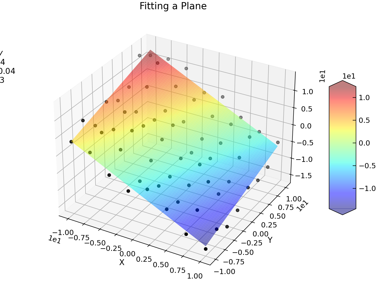
Fitting Tricks
Fitting 3D Data
Stoner.Data.curve_fit() can also be used to fit 3D (or higher order) data - i.e. where there are two independent
variables. In order to do this, the xcol parameter needs to be an iterable (e.g. list or tuple or array), and
the function to be fitted needs to take a tuple of scalars or arrays as the first argument. The following example
illustrates this by fitting a plane to a collection of points in 3D space.
"""Use curve_fit to fit a plane to some data."""

import matplotlib.cm as cmap
from numpy import array, column_stack, linspace, meshgrid
from numpy.random import normal, seed

from Stoner import Data

seed(12345)  # Ensire consistent random numbers!


def plane(coord, a, b, c):
    """Function to define a plane."""
    x, y = coord.T
    return c - (x * a + y * b)


coeefs = [1, -0.5, -1]
col = linspace(-10, 10, 8)
X, Y = meshgrid(col, col)
Z = plane(array([X, Y]).T, *coeefs) + normal(size=X.shape, scale=2.0)
d = Data(
    column_stack((X.ravel(), Y.ravel(), Z.ravel())),
    filename="Fitting a Plane",
    setas="xyz",
)

d.column_headers = ["X", "Y", "Z"]
d.plot_xyz(plotter="scatter", title=None, griddata=False, color="k")

popt, pcov = d.curve_fit(plane, [0, 1], 2, result=True)
col = linspace(-10, 10, 128)
X, Y = meshgrid(col, col)
Z = plane(array([X, Y]).T, *popt)
e = Data(
    column_stack((X.ravel(), Y.ravel(), Z.ravel())),
    filename="Fitting a Plane",
    setas="xyz",
)
e.column_headers = d.column_headers

e.plot_xyz(linewidth=0, cmap=cmap.jet, alpha=0.5, figure=d.fig)

txt = "$z=c-ax+by$\n"
txt += "\n".join([d.format(f"plane:{k}", latex=True) for k in ["a", "b", "c"]])

ax = d.axes[0]
ax.text(-30, -10, 10, txt)

Fitting to Minimize a Function
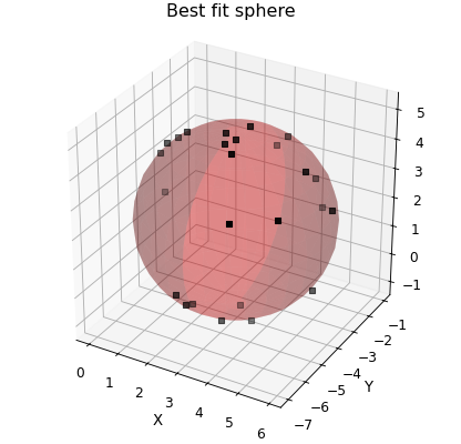
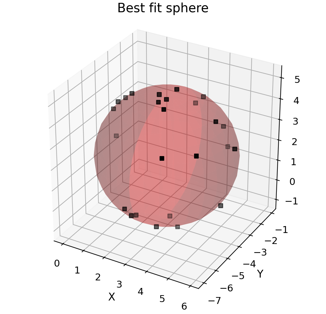
If ycol is a numpy array of the same length as the data then the values of ycol are assumed to be the points to fit rather than index of a column. This is useful if the function you want to fit can be written as \(f(x_1,x_2,\cdots ,x_n)=0\). In thus case pass xcol a list or tuple of columns that make up \(x_1,x_2,\cdots ,x_n\) and make your function take a tuple of 1D-arrays and pass ycol as an array of zeros. For example:
"""Fit a sphere with curve_fit."""

import matplotlib.pyplot as plt
from numpy import (
    column_stack,
    cos,
    linspace,
    meshgrid,
    ones_like,
    pi,
    sin,
    zeros_like,
)
from numpy.random import normal, seed, uniform

from Stoner import Data

seed(12345)  # Ensure consistent random numbers!


def transform(r, q, p):
    """Converts from spherical to cartesian coordinates."""
    x = r * cos(q) * cos(p)
    y = r * cos(q) * sin(p)
    z = r * sin(q)
    return x, y, z


def sphere(coords, a, b, c, r):
    """Returns zero if (x,y,z) lies on a sphere centred at (a,b,c) with radius r."""
    x, y, z = coords.T
    return (x - a) ** 2 + (y - b) ** 2 + (z - c) ** 2 - r**2


# Create some points approximately spherical distribution
num = 25
q = uniform(low=-pi / 2, high=pi / 2, size=num)
p = uniform(low=0, high=2 * pi, size=num)
r = normal(loc=3.0, size=num, scale=0.2)

x, y, z = transform(r, q, p)

x += 3.0
y -= 4.0
z += 2.0

# Construct the  DataFile object
d = Data(
    column_stack((x, y, z)),
    setas="xyz",
    filename="Best fit sphere",
    column_headers=["X", "Y", "Z"],
)
d.template.fig_width = 5.2
d.template.fig_height = 5.0  # Square aspect ratio
d.plot_xyz(plotter="scatter", marker=",", griddata=False)
d.set_box_aspect((1, 1, 1.0))  # Passing through to the current axes
# curve_fit does the hard work
popt, pcov = d.curve_fit(sphere, (0, 1, 2), zeros_like(d.x), result=True)

# This manually constructs the best fit sphere
a, b, c, r = popt
p = linspace(-pi / 2, pi / 2, 16)
q = linspace(-pi, pi, 31)
P, Q = meshgrid(p, q)
R = ones_like(P) * r
x, y, z = transform(R, Q, P)
x += a
y += b
z += c

ax = d.axes[0]
ax.plot_surface(
    x, y, z, rstride=1, cstride=1, color=(1.0, 0.0, 0.0, 0.25), linewidth=0
)
plt.draw()
d.annotate_fit(sphere, prefix="sphere", x=-4.5, y=-4, z=3)
Other Recipes
Extract X-Y(Z) from X-Y-Z data
In a number of measurement systems the data is returned as 3 parameters X, Y and Z and one wishes to extract X-Y as a function of constant Z. For example, I-V sweeps as a function of gate voltage V:sub:G. Assuming we have a data file with columns Current, Voltage,*Gate*:
d=DataFile('data.txt')
t=d
for gate in d.unique('Gate'):
    t.data=d.search('Gate',gate)
    t.save('Data Gate='+str(gate)+'.txt')
The first line opens the data file containing the I-V(V_G) data. The second
creates a temporary copy of the Stoner.Core.DataFile object - ensuring that we get a copy of
all metadata and column headers. The for loop iterates over all unique
values of the data in the gate column and then inside the for loop, searches for
the corresponding I-V data, sets it as the data of the temporary DataFile and
then saves it.
Mapping X-Y-Z data to Z(X,Y) data
In a similar fashion to the previous section, where data has been recorded with fixed values of X and Y eg I measured for fixed V and V_, it can be useful to map the data to a matrix.:
d=DataFile('Data,.txt')
t=d
for gate in d.unique('Gate'):
   t=t+d.search('Gate',gate)[:,d.find_col('Current')]
t.column_headers=['Bias='+str(x) for x in d.unique('Voltage')]
t.add_column(d.unique('Gate'),'Gate Voltage',0)
The start of the script follows the previous section, however this time in the
for loop the addition operator is used to add a single row to the temporary
Stoner.Core.DataFile t. In this case we are using the utility method
Stoner.Core.DataFile.find_col() to find the index of the column with the current
data. After the for loop we set the column headers in t and then insert
an additional column at the start with the gate voltage values.
The matrix generated by this code is suitable for feeding directly into
Stoner.plot.PlotMixin.plot_matrix(), however, the same plot could be generated
directly from the Stoner.plot.PlotMixin.plot_xyz() method too.
Sampling a A 3D Surface function
Suppose you have a function Z(x,y) that is defined over a range -X0..+X0 and
-Y0..y0 and want to quickly get a view of the surface. This problem can be easily done
by creating a random distribution of (x,y) points, evaluating the function and then
using the PlotFile methods to generate the surface.:
from Stoner import Data
from numpy import uniform

samples=5000

surf=Data()
surf&=uniform(-X0,X0,samples)
surf&=uniform(-Y0,Y0,samples)
surf.setas="xy"
surf&=Z(surf.x,surf.y)
surf.setas="xyz"
surf.plot() # or surf.plot(cstride=1,rstride=1,linewidth=0) for finer detail.
Quickly Sectioning a 3D dataset
We often model the magnetic state in our experiments using a variety of micromagnetic modelling codes, such OOMMF or MuMax. When modelling a 3D system, it is often useful to be able to examine a cross-section of the simulation. The Stoner package provides tools to quickly examine the output data:
from Stoner.FileFormats import OVFFile # reads OOMMF vector field files
import Stoner.plot
p=SP.PlotFile('my_simulation.ovf')
p.setas="xyzuvw"
p=p.section(z=10.5) # Take a slice in the xy plane where z is 10.5 nm
p.plot() # A 3D plot with cones
p.setas="xy.uvw"
p.plot() # a 2D colour wheel plot with triangular glyphs showing vector direction.