vftEquation

Stoner.analysis.fitting.models.thermal.vftEquation(x, A, DE, x_0)

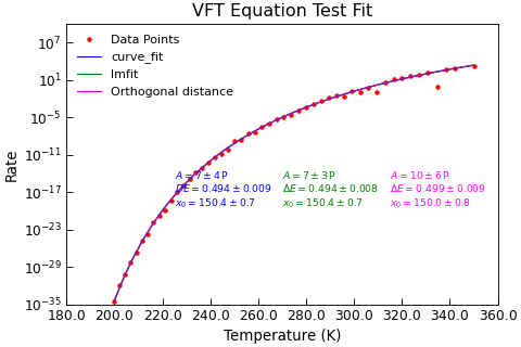
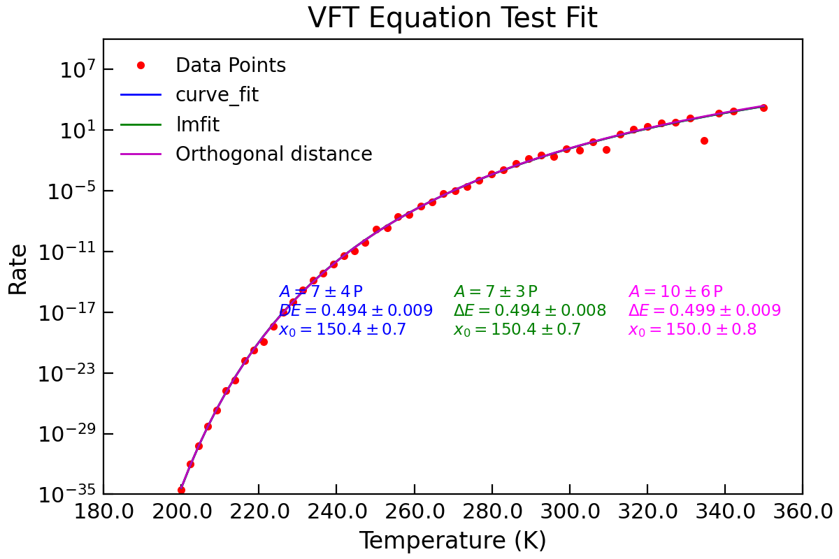
Vogel-Flucher-Tammann (VFT) Equation without T dependent prefactor.

Parameters:

• x (float) – Temperature in K

• A (float) – Prefactror (not temperature dependent)

• DE (float) – Energy barrier in eV

• x_0 (float) – Offset temperature in K

Returns:

Rates according the VFT equation.

The VFT equation is defined as as \(\tau = A\exp\left(\frac{DE}{x-x_0}\right)\) and represents a modified form of the Arrenhius distribution with a freezing point of \(x_0\).

Example

"""Example of Arrhenius Fit."""
from numpy import logspace, log10
from numpy.random import normal

from Stoner import Data
from Stoner.analysis.fitting.models.thermal import vftEquation, VFTEquation

# Make some data
T = logspace(log10(200), log10(350), 51)
params = (1e16, 0.5, 150)
noise = 0.5
R = vftEquation(T, *params) * normal(size=len(T), scale=noise, loc=1.0)
dR = vftEquation(T, *params) * noise
d = Data(T, R, dR, setas="xy.", column_headers=["T", "Rate"])

# Plot the data points.
d.plot(fmt="r.", label="Data Points")

# Turn on the sigma column (error bars look messy on plot due to logscale)
d.setas[2] = "e"

# Curve_fit on its own
d.curve_fit(vftEquation, p0=params, result=True, header="curve_fit")

# lmfit uses some guesses
p0 = params
d.lmfit(VFTEquation, result=True, header="lmfit")

# Plot these results too
d.setas = "x..yy"
d.plot(fmt=["b-", "g-"])
# Annotate the graph
d.annotate_fit(
    vftEquation,
    x=0.25,
    y=0.35,
    fontdict={"size": "x-small", "color": "blue"},
    mode="eng",
)
d.annotate_fit(
    VFTEquation,
    x=0.5,
    y=0.35,
    prefix="VFTEquation",
    fontdict={"size": "x-small", "color": "green"},
    mode="eng",
)

# reset the columns for the fit
d.setas = "xye.."
# Now do the odr fit (will overwrite lmfit's metadata)
d.odr(VFTEquation, result=True)
d.setas = "x4.y"

# And plot and annotate
d.plot(fmt="m-", label="Orthogonal distance")
d.annotate_fit(
    VFTEquation,
    x=0.75,
    y=0.35,
    fontdict={"size": "x-small", "color": "magenta"},
    mode="eng",
)

# Finally tidy up the plot a bit
d.yscale = "log"
d.ylim = (1e-35, 1e10)
d.title = "VFT Equation Test Fit"
d.ylabel = "Rate"
d.xlabel = "Temperature (K)"

(png, hires.png, pdf)