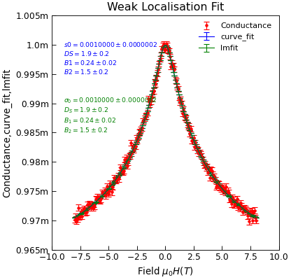
wlfit

Stoner.analysis.fitting.models.e_transport.wlfit(B, s0, DS, B1, B2)

Implement the Weak localisation fitting function.

Parameters:

• B (array) – mag. field

• s0 (float) – zero field conductance

• DS (float) – scaling parameter

• B1 (float) – elastic characteristic field (B1)

• B2 (float) – inelastic characteristic field (B2)

Returns:

Conductance vs Field for a weak localisation system

Notes

2D WL model as per Wu et al PRL 98, 136801 (2007), Porter et al PRB 86, 064423 (2012)

Example

"""Test Weak-localisation fitting."""
from copy import copy

from numpy import linspace, ones_like
from numpy.random import normal

from Stoner import Data
from Stoner.analysis.fitting.models.e_transport import WLfit, wlfit

B = linspace(-8, 8, 201)
params = [1e-3, 2.0, 0.25, 1.4]
G = wlfit(B, *params) + normal(size=len(B), scale=5e-7)
dG = ones_like(B) * 5e-7
d = Data(
    B,
    G,
    dG,
    setas="xye",
    column_headers=["Field $\\mu_0H (T)$", "Conductance", "dConductance"],
)

d.curve_fit(wlfit, p0=copy(params), result=True, header="curve_fit")

d.setas = "xye"
d.lmfit(WLfit, result=True, header="lmfit")

d.setas = "xyeyy"
d.plot(fmt=["r.", "b-", "g-"])

d.annotate_fit(
    wlfit, x=0.05, y=0.75, fontdict={"size": "x-small", "color": "blue"}
)
d.annotate_fit(
    WLfit,
    x=0.05,
    y=0.5,
    fontdict={"size": "x-small", "color": "green"},
    prefix="WLfit",
)
d.title = "Weak Localisation Fit"

(png, hires.png, pdf)