Data.lmfit
- Data.lmfit(model, xcol=None, ycol=None, p0=None, sigma=None, **kwargs)
Wrap the lmfit module fitting.
- Parameters:
datafile (Data) – Data object to work with if not being used as a bound method.
model (lmfit_mod.Model) – An instance of an lmfit_mod.Model that represents the model to be fitted to the data
xcol (index or None) – Columns to be used for the x data for the fitting. If not givem defaults to the
Stoner.Core.DataFile.setasx columnycol (index or None) – Columns to be used for the y data for the fitting. If not givem defaults to the
Stoner.Core.DataFile.setasy column
- Keyword Arguments:
p0 (list, tuple, array or callable) – A vector of initial parameter values to try. See the notes in
Stoner.Data.curve_fit()for more details.sigma (index) – The index of the column with the y-error bars
bounds (callable) – A callable object that evaluates true if a row is to be included. Should be of the form f(x,y)
result (bool) – Determines whether the fitted data should be added into the DataFile object. If result is True then the last column will be used. If result is a string or an integer then it is used as a column index. Default to None for not adding fitted data
replace (bool) – Inidcatesa whether the fitted data replaces existing data or is inserted as a new column (default False)
header (string or None) – If this is a string then it is used as the name of the fitted data. (default None)
scale_covar (bool) – whether to automatically scale covariance matrix (leastsq only)
output (str, default "fit") – Specify what to return.
**kwargs – Other arguments to pass to curve_fit_result or initial p0 values for curve_fit.
- Returns:
( various ) –
- The return value is determined by the output parameter. Options are
- ”fit” just the
lmfit_mod.Model.ModelFitinstance that contains all relevant information about the fit.
- ”fit” just the
- ”row” just a one dimensional numpy array of the fit parameters interleaved with their
uncertainties
”full” a tuple of the fit instance and the row.
- ”data” a copy of the
Stoner.Core.DataFileobject with the fit recorded in the emtadata and optionally as a column of data.
- ”data” a copy of the
See also
Note
If p0 is fed a 2D array, then it assumed that you want to calculate \(\chi^2\) for different starting parameters with some variables fixed. In this mode, fitting is carried out repeatedly with each row representing one attempt with different values of the parameters. In this mode the return value is a 2D array whose rows correspond to the inputs to the rows of p0, the columns are the fitted values of the parameters with an additional column for \(\chi^2\).
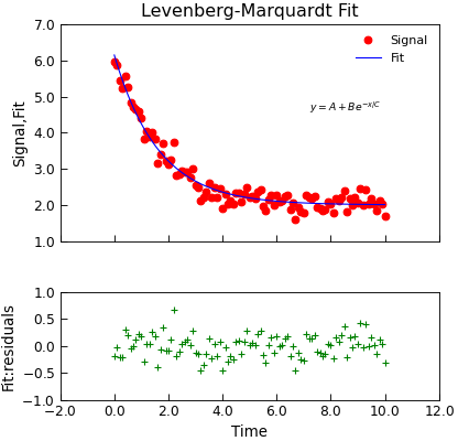
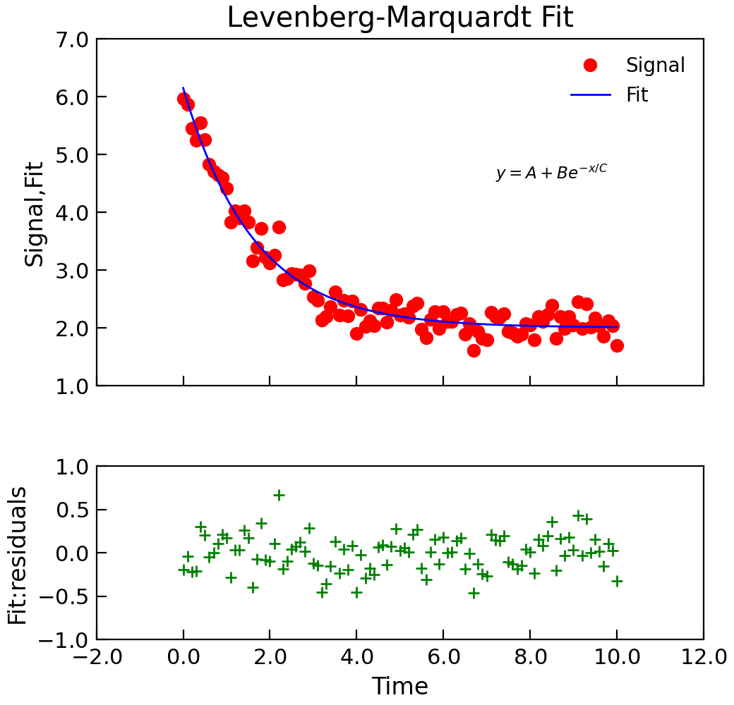
Example
"""Simple use of lmfit to fit data."""

from numpy import exp, linspace, random

from Stoner import Data

random.seed(12345)  # Ensure Consistent Random numbers
# Make some data
x = linspace(0, 10.0, 101)
y = 2 + 4 * exp(-x / 1.7) + random.normal(scale=0.2, size=101)

d = Data(x, y, column_headers=["Time", "Signal"], setas="xy")


# Do the fitting and plot the result
def func(x, A, B, C):
    """Simple fitting function."""
    return A + B * exp(-x / C)


fit = d.lmfit(
    func,
    result=True,
    header="Fit",
    A=1,
    B=1,
    C=1,
    residuals=True,
    output="report",
)

# Reset labels
d.labels = []

# Make nice two panel plot layout
ax = d.subplot2grid((3, 1), (2, 0))
d.setas = "x..y"
d.plot(fmt="g+")
d.title = ""

ax = d.subplot2grid((3, 1), (0, 0), rowspan=2)
d.setas = "xyy"
d.plot(fmt=["ro", "b-"])
d.xticklabels = [[]]
d.xlabel = ""

# Annotate plot with fitting parameters
d.annotate_fit(func, prefix="Model", x=7.2, y=3, fontdict={"size": "x-small"})
text = r"$y=A+Be^{-x/C}$" + "\n\n"
d.text(7.2, 3.9, text, fontdict={"size": "x-small"})
d.title = "Levenberg-Marquardt Fit"
