Analysing Data Files

Normalising and Basic Maths Operations

Several methods are provided to assist with common data fitting and preparation tasks, such as normalising columns, adding and subtracting columns.:

a.normalise('data','reference',header='Normalised Data',replace=True)
a.normalise(0,1)
a.normalise(0,3.141592654)
a.normalise(0,a2.column(0))

The AnalysisMixin.normalise() method simply divides the data column by the reference column. By default the normalise method replaces the data column with the new (normalised) data and appends ‘(norm)’ to the column header. The keyword arguments header and replace can override this behaviour. The third variant illustrates normalising to a constant (note, however, that if the second argument is an integer it is treated as a column index and not a constant). The final variant takes a 1D array with the same number of elements as rows and uses that to normalise to. A typical example might be to have some baseline scan that one is normalising to.:

a.subtract('A','B'm header="A-B",replace=True)
a.subtract(0,1)
a.subtract(0,3.141592654)
a.subtract(0,a2.column(0))

As one might expect form the name, the AnalysisMixin.subtract() method subtracts the second column form the first. Unlike AnalysisMixin.normalise() the first data column will not be replaced but a new column inserted and a new header (defaulting to ‘column header 1 - column header 2’) will be created. This can be overridden with the header and replace keyword arguments. The next two variants of the AnalysisMixin.subtract() method work in an analogous manner to the AnalysisMixin.normalise() methods. Finally the AnalysisMixin.add() method allows one to add two columns in a similar fashion:

a.add('A','B',header='A plus B',replace=False)
a.add(0,1)
a.add(0,3.141592654)
a.add(0,a2.column(0))

For completeness we also have:

a.divide('A','B',header='A/B', replace=True)
a.multiply('A','B',header='A*B', replace=True)

with variants that take either a 1D array of data or a constant instead of the B column index.

The final variant for these channel operations is the AnalysisMixin.diffsum() which takes the ratio of the difference over the sum of two channels. This is typically used to calculate asymmetry parameters.:

a.diffsum('I+','I-')

Of course, these elementary operations might look rather pointless given how easy it is to extract single columns of data and then add them to a Stoner.Core.Data object, however if the channels are specified as a tuple of two elements, then it is taken as a channel of data and a second channel of uncertainties. The uncertainty calculation is then propagated correctly for the maths operations. This is particularly useful for the AnalysisMixin.diffsum() method where the error propagation is not entirely trivial.

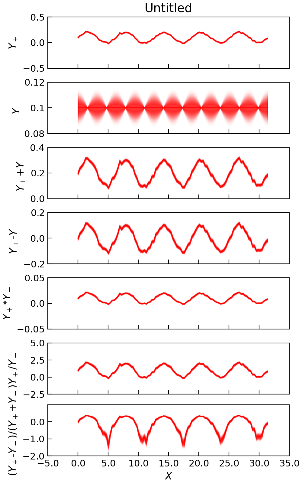
"""Demonstrate Channel math operations."""
from numpy import linspace, ones_like, sin, cos, pi
from numpy.random import normal, seed

from Stoner import Data
from Stoner.plot.utils import errorfill

seed(12345)  # Ensure consistent random numbers!
x = linspace(0, 10 * pi, 101) + 1e-9
e = 0.01 * ones_like(x)
y = 0.1 * sin(x) + normal(size=len(x), scale=0.01) + 0.1
e2 = 0.01 * cos(x)
y2 = 0.1 * ones_like(x)
d = Data(
    x,
    y,
    e,
    y2,
    e2,
    column_headers=["$X$", "$Y_+$", r"$\delta Y_+$", "$Y_-$", r"$\delta Y_-$"],
    setas="xyeye",
)

a = tuple(d.column_headers[1:3])
b = tuple(d.column_headers[3:5])

d.add(a, b, replace=False)
d.subtract(a, b, replace=False)
d.multiply(a, b, replace=False)
d.divide(a, b, replace=False)
d.diffsum(a, b, replace=False)
d.setas = "xyeyeyeyeyeyeye"
d.plot(
    multiple="panels",
    plotter=errorfill,
    color="red",
    alpha_fill=0.2,
    figsize=(5, 8),
)

(png, hires.png, pdf)

Splitting Data Up

One might wish to split a single data file into several different data files each with the rows of the original that have a common unique value in one data column, or for which some function of the complete row determines which datafile each row belongs in. The AnalysisMixin.split() method is useful for this case.:

a.split('Polarisation')
a.split('Temperature',lambda x,r:x>100)
a.split(['Temperature','Polarisation'],[lambda x,r:x>100,None])

In these examples we assume the AnalysisMixin has a data column ‘Polarisation’ that takes two (or more) discrete values and a column ‘Temperature’ that contains numbers above and below 100.

The first example would return a Stoner.Folders.DataFolder object containing two separate instances of AnalysisMixin which would each contain the rows from the original data that had each unique value of the polarisation data. The second example would produce a Stoner.Folders.DataFolder object containing two AnalysisMixin objects for the rows with temperature above and below 100. The final example will result in a Stoner.Folders.DataFolder object that has two groups each of which contains AnalysisMixin objects for each polarisation value.

More AnalysisMixin Functions

Applying an arbitrary function through the data

AnalysisMixin.apply():

a.apply(func, col, replace = True, header = None)

Here func is an arbitrary function that will take a complete row in the form of a numpy 1D array, col is the index of a column at which the resulting data is to be inserted or overwrite the existing data (depending on the values of replace and header).

Basic Data Inspection

AnalysisMixin.max() and AnalysisMixin.min():

a.max(column)
a.min(column)
a.max(column,bounds=labda x,y:y[2]>1 and y[2]<10)
a.min(column,bounds=labda x,y:y[2]>1 and y[2]<10)

Hopefully all of the above are fairly obvious ! In the last two cases, one can use a function to limit the search to particular rows (eg to search for the maximum y value subject to some constraint in x). One important point to note is that the routines return a tuple of two numbers, the maximum (or minimum) and the row number where the maximum or minimum was found.

There are a couple of related functions to help here:

a.span(column)
a.span(column, bounds=lambda x,y:y[2]>100)
a.clip(column,(max_v,min_v)
a.clip(column,b.span(column))

The AnalysisMixin.span() method simply returns a tuple of minimum and maximum values within either the whole column or bounded data. Internally this is just calling the AnalysisMixin.max() and AnalysisMixin.min() methods. The AnalysisMixin.clip() method deletes rows for which the specified column as a value that is either larger or smaller than the maximum or minimum value within the second argument. This allows one to specify either a tuple – eg the result of the AnalysisMixin.span() method, or a complete list as in the last example above. Specifying a single float would have the effect of removing all rows where the column didn’t equal the float value. This is probably not a good idea…

It is worth pointing out that these functions will respect the existing mask on the data unless the bounds parameter is set, in which case the mask is temporarily discarded in favour of one generated from the bounds expression. This can be worked around, however, as the parameter passed to the bounds function is itself a masked array and thus one can include a test of the mask in the bounds function:

a.span(column,bounds=lambda x,y:y[2]>10 or not numpy.any(y.mask))

Data Reduction Methods

AnalysisMixin offers a number of methods to assist in data reduction and data processing.

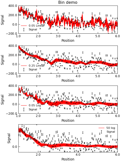
(Re)Binning Data

Data binning is the process of taking approximately continuous (x,y) data and grouping them into “bins” of specified x, and average y. Since this is a data averaging process, the statistical variation in y values is reduced, at the expense of a loss of resolution in x.

AnalysisMixin provides a simple AnalysisMixin.bin() method that can re-bin data:

(x_bin,y_bin,dy)=a.bin(xcol="Q",ycol="Counts",bins=100,mode="lin")
(x_bin,y_bin,dy)=a.bin(xcol="Q",ycol="Counts",bins=0.02,mode="log",yerr="dCounts")
(x_bin,y_bin,dy)=a.bin(mode="log",bins=0.02,bin_start=0.001,bin_stop=0.1)

The mode parameter controls whether linear binning or logarithmic binning is used. The bins parameter is either an integer in which case it specifies the number of bins to be used, or a float in which case it specifies the bin width. For logarithmic binning the bin width for bin n is defined as \(x_n * w\) with \(w\) being the bin width parameter. Thus the bin boundaries are at \(x_n\) and \(x_{n+1}=x_n(1+w)\) whilst the bin centre is at \(x_n(1+\frac{w}{2})\). If a number of bins is specified in logarithmic mode then the bin boundaries are set from equal logspace boundaries.

If the keyword yerr is supplied then the y values in each bin are weighted by their respective error bars when calculating the mean. In this case the error bar on the bin bceomes the quadrature sum of the individual error bars on each point included in the bin. If yerr is nopt specified, then the error bar is the standard error in the y points in the bin and the y value is the simple mean of the data.

If xcol and/or ycol are not specified, then they are looked up from the Stoner.Core.DataFile.setas attribute. In this case, the yerr is also taken from this attribute if not specified separately.

IF the keyword clone is supplied and is False, four 1D numpy arrays are returned, representing the x, y and y-errors for the new bins and the number of points averaged into each bin.. If clone is True or not provided, AnalysisMixin.bin() returns a clone of the current data file with its data (and column headers) replaced with the newly binned data.

"""Re-binning data example."""
from Stoner import Data
from Stoner.plot.utils import errorfill

d = Data("Noisy_Data.txt", setas="xy")

d.template.fig_height = 6
d.template.fig_width = 8
d.figure(figsize=(6, 8), no_axes=True)
d.subplot(411)

e = d.bin(bins=0.05, mode="lin")
f = d.bin(bins=0.25, mode="lin")
d.setas = "xye"
g = d.bin(bins=0.05, mode="log")
h = d.bin(bins=50, mode="log")

for i, (binned, label) in enumerate(
    zip([e, f, g, h], ["0.05 Linear", "0.25 Linear", "0.05 Log", "50 log"])
):
    binned.subplot(411 + i)
    d.plot(fmt="k,", capsize=2.0)
    binned.fig = d.fig
    binned.plot(plotter=errorfill, label=label, color="red")

    d.xlim = (1, 6)
    d.ylim(-100.0, 400)
    d.title = "Bin demo" if i == 0 else ""

(png, hires.png, pdf)

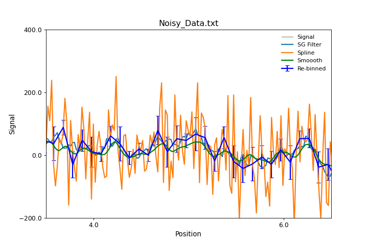
Smoothing and Filtering Data

As experimental data normally includes noise in some form, it is useful to be able to filter and smooth data to better see underlying trends. The Stoner package offers a number of approaches to filtering data.

• Smoothing by convoluting with a window

  This is a powerful method of smoothing data by constructing an appropriate length and shape of ‘window function’ that is then convulted with the data so that every point becomes some form of weighted average of surrounding points as defined by the window function. This is handled by the AnalysisMixin.smooth() method.:

  d.smooth("boxcar",size=10)
  d.smooth(("gaussian",1.5),size=0.4,result=True,replace=False,header="Smoothed data")
  

  In both these examples, the data to be smoothed is determined from the Stoner.Core.DataFile.setas attribute. The first argument is passed to scipy.signal.get_window() to define the window function. The size argument can either be an integer to specify the number of rows in the window, or a float to specify the size of the window in terms of the x data. In the latter case, the data is first reinterpolated to an evenly space set in terms of the x-column and then smoothed and then reinterpolated back to the original x data coordinates.

  Warning

  This will fail for hysteretic data. In this case it would be better to use an integer size argument and to ensure the data is evenly spaced to start with.

  The result and replace arguments are passed through to Stoner.Core.DataFile.add_column() unless replace is False in which case, the smoothed data is passed back as the return value and the current AnalysisMixin is left unmodified.

• Savitzky-Golay filtering

  This is a common filtering technique, particularly for spectroscopic data as it is good at keeping major peak locations and widths. In essence it is equivalent to least-squares fitting a low order polynomial to a window of the data and using the co-effienicents of the fitting polynomail to determine the smoothed (or differentiated) data. This is impletemented as AnalysisMixin.SG_Filter() method.

• Spline

  An alternative approach is to use a smoothing spline to fit the data locally. Depending on the spline smoothing setting this will create a function that is continuous in both value and derivative that approaches the data. Unlike Savotzky- Golay filtering it cannot be used to calculate a derivative easily, but it can handle y data with uncertainties. It is implemented as the AnalysisMixin.spline() method.

• Rebinning

  As ullustrated above, rebinning the data is a common way for reducing noise by combining several data points. This is simple and effective, but does reduce the length of the data !

All three approaches are illustrated in the excample below:

"""Smoothing Data methods example."""
import matplotlib.pyplot as plt

from Stoner import Data

fig = plt.figure(figsize=(9, 6))

d = Data("Noisy_Data.txt", setas="xy")

d.fig = fig
d.plot(color="grey")
# Filter with Savitsky-Golay filter, linear over 7 ppoints
d.SG_Filter(result=True, points=11, header="S-G Filtered")
# Filter with cubic splines
d.spline(result=True, order=3, smoothing=4, header="Spline")
# Rebin data
d.smooth("hamming", size=0.2, result=True, header="Smoothed")

d.plot(0, "S-G Filtered", lw=2, label="SG Filter")
d.plot(0, "Spline", lw=2, label="Spline")
d.plot(0, "Smooth", lw=2, label="Smoooth", color="green")

d2 = d.bin(bins=100, mode="lin")
d2.fig = d.fig
d2.plot(lw=2, label="Re-binned", color="blue")
d2.xlim(3.5, 6.5)
d2.ylim(-200.0, 400.0)

(png, hires.png, pdf)

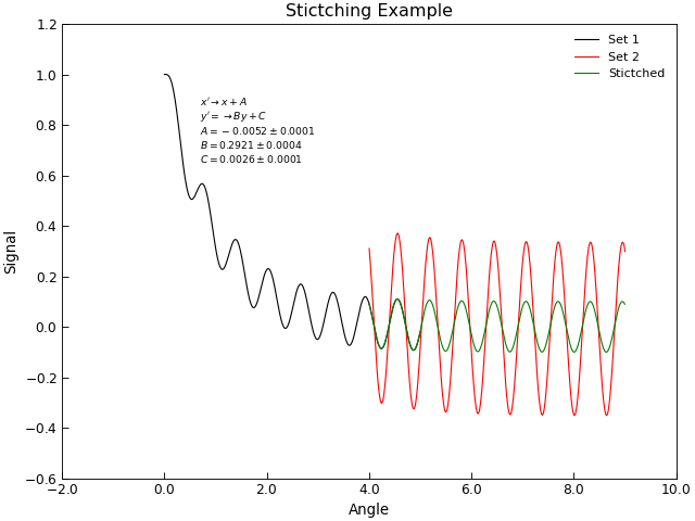
Stitching Datasets together

Sometimes a data set is obtained by joing together several separate sets of data, for example, joinging several scans over different angular or energy ranges to make a single combinaed scan. In the ideal world, these scans could simple be joing together (e.g. by using the + operator), in practise one often finds that there are systematic changes in scaling or offsets between individual scans. The task of stitching data sets together then becomes one of finding the best mapping between two sets of (x,y) points that are nominally the same. AnalysisMixin provides a AnalysisMixin.stitch() method to facilitate this.

"""Scale data to stitch it together."""
import matplotlib.pyplot as plt

from Stoner import Data
from Stoner.Util import format_error

# Load and plot two sets of data
s1 = Data("Stitch-scan1.txt", setas="xy")
s2 = Data("Stitch-scan2.txt", setas="xy")
s1.plot(label="Set 1")
s2.fig = s1.fig
s2.plot(label="Set 2")
# Stitch scan 2 onto scan 1
s2.stitch(s1)

s2.plot(label="Stictched")
s2.title = "Stictching Example"

# Tidy up the plot by adding annotation fo the stirching co-efficients
labels = ["A", "B", "C"]
txt = []
lead = r"$x'\rightarrow x+A$" + "\n" + r"$y'=\rightarrow By+C$" + "\n"
for l, v, e in zip(
    labels, s2["Stitching Coefficients"], s2["Stitching Coefficient Errors"]
):
    txt.append(format_error(v, e, latex=True, prefix=l + "="))
plt.text(0.7, 0.65, lead + "\n".join(txt), fontdict={"size": "x-small"})
plt.draw()

(png, hires.png, pdf)

The stitch method can be fine tuned by specifying the possible scaling and shifting operations, overlap region to use or even a custom stiching transofmration function:

s2.stitch(s1,mode="shift x")
s2.stitch(s1,mode="scale y, shift x",overlap=(3.0,5.0))
s2.stitch(s1,func=my_stitcher,p0=[3.14,2.54,2.0])

In these examples, the x and y columns of scan2 are modified to give the best possible match to scan1. If xcol or ycol are not given then the default x and y columns as set py the Stoner.Core.DataFile.setas attribute.

The mode keyword can be used to specify the types of scaling operations that are to be allowed. The defaults are to shoft both x and y by an offset value and to rescale the y data by some factor. If even more control of the transformation is needed, the func keyword and p0 keyword can be used to provide an alternative transformation function and initial guesses to its parameters. The profotype for the transformation function should be:

def my_stitcher(x,y,p1,p2,p3...,pn):
    ...
    return (mapped_x,mapped_y)

In addition to changing the X and Y data in the current AnalysisMixin instance, two new metadata keys, Stitching Coefficient and Stitching Coefficient Errors, with the co-efficients used to modify the scan data.

Thresholding, Interpolating and Extrapolation of Data

Thresholding data is the process of identifying points where y data values cross a given limit (equivalently, finding roots for \(y=f(x)-y_{threshold}\)). This is carried out by the AnalysisMixin.threshold() method:

a.threshold(threshold, col="Y-data", rising=True, falling=False,all_vals=False,xcol="X-data")
a.threshold(threshold)

If the parameters col and xcol are not given, they are determined by the Stoner.Core.DataFile.setas attribute. The rising and falling parameters control whether the y values are rising or falling with row number as they pass the threshold and all_vals determines whether the method returns just the first threshold or all thresholds it can find. The values returned are mapped to the x-column data if it is specified. The thresholding uses just a simple two point linear fit to find the thresholds.

Interpolating data finds values of y for points x that lie between data points. The AnalysisMixin.interpolate() provides a simple pass-through to the scipy routine scipy.optimize.interp1d():

a.interpolate(newX,kind='linear', xcol="X-Data")

The new values of X are set from the mandatory first argument. kind can be either “linear” or “cubic” whilst the xcol data can be omitted in which case the Stoner.Core.DataFile.setas attribute is used. The method will return a new set of data where all columns are interpolated against the new values of X.

The AnalysisMixin.interpolate() method will return values that are obtained from ‘joining the dots’ - which is appropriate if the uncertainties (and hence scatter) in the data is small. With more scatter in the data, it is better to use some locally fitted spline function to interpolate with. The AnalysisMixin.spline() function can be used for this.:

d.spline("X-Data","Y-Data",header="Spline Data",order=3,smoothing=2.0,replace=True)
d.spline("X-Data","Y-Data",header="Spline Data",order=2,smoothing=2.0,replace="Extra")
new_y=d.spline("X-Data","Y-Data",order=2,smoothing=2.0,replace=False)
spline=d.spline("X-Data","Y-Data",order=2,smoothing=2.0,replace=None)

The order keyword gives the polynomial order of the spline function being fitted. The smoothing factor determines how closely the spline follows the data points, with a smoothing*=0.0 being a strict interpolation. The *repalce argument controls what the return value from the AnalysisMixin.spline() method returns. IF replace is True or a column index, then the new data is added as a column of the Data, possibly replacing the current y-data. If replace is False, then the new y-data is returned, but the existing data is unmodified. Finally, if replace is None, then the AnalysisMixin.spline() method returns a scipy.interpolate.UnivararateSpline object that can be used to evaluate the spline at arbitrary locations, including extrapolating outside the range of the original x data.

Extrapolation is, of course, a dangerous, operation when applied to data as it is essentially ‘inventing’ new data. Extrapolating fromt he spline function, whislt possible, is a little tricky and in many cases the AnalysisMixin.extrapolate() method is likely to be more successful. AbnalyseFile.extrapolate() works by fitting a function over a window in the data and using the fit function to predict nearby values. Where the new values lie within the range of data, this is strictly a form of interpolation and the window of data fitted to the extrpolation function is centred around the new x-data point. As the new x-data point approaches and passes the limits of the existing data, the window used to provide the fit function runs up to and stops at the limit of the supplied data. Thus when extrapolating, the new values of data are increasingly less certain as one moves further from the end of the data.

"""Extrapolate data example."""
from numpy import linspace, ones_like, column_stack, exp, sqrt
from numpy.random import normal, seed
import matplotlib.pyplot as plt

from Stoner import Data
from Stoner.plot.utils import errorfill

seed(1245)  # Ensure consistent random numbers
x = linspace(1, 10, 101)
d = Data(
    column_stack(
        [
            x,
            (2 * x**2 - x + 2) + normal(size=len(x), scale=2.0),
            ones_like(x) * 2,
        ]
    ),
    setas="xye",
    column_headers=["x", "y", "errors"],
)

extra_x = linspace(8, 15, 11)

y4 = d.extrapolate(
    extra_x,
    overlap=200,
    kind=lambda x, A, C: A * exp(x / 10) + C,
    errors=lambda x, Aerr, Cerr, popt: sqrt(
        (Aerr * exp(x / popt[1])) ** 2 + Cerr**2
    ),
)
y3 = d.extrapolate(extra_x, overlap=80, kind="cubic")
y2 = d.extrapolate(extra_x, overlap=3.0, kind="quadratic")
y1 = d.extrapolate(extra_x, overlap=1.0, kind="linear")

d.plot(fmt="k.", capsize=2.0)
d.title = "Extrapolation Demo"

errorfill(
    extra_x, y4[:, 0], color="orange", yerr=y4[:, 1], label="Arg. Function"
)

errorfill(
    extra_x, y3[:, 0], color="red", yerr=y3[:, 1], label="Cubic Extrapolation"
)

errorfill(
    extra_x,
    y2[:, 0],
    color="green",
    yerr=y2[:, 1],
    label="Quadratic Extrapolation",
)
errorfill(
    extra_x, y1[:, 0], color="blue", yerr=y1[:, 1], label="Linear Extrapolation"
)
plt.legend(loc=2)

(png, hires.png, pdf)

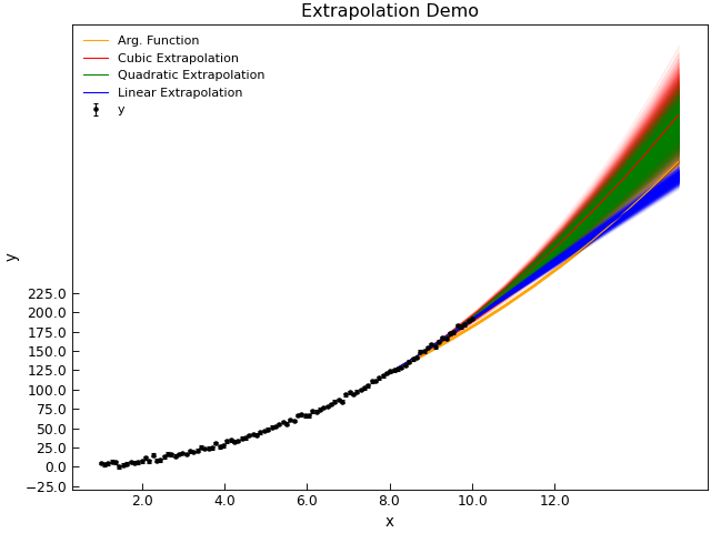
Extrapolation is of course most successful if one has a physical model that should describe the data. To allow for this, you can pass an arbitrary fitting function as the kind parameter.

Whilst interpolation will tell you the

Smoothing and Differentiating Data

Smoothing and numerical differentation are carried out using the Savitsky-Golay filtering function. Whilst not the most sophisticated algorithm it is reasonably easy to implement and simple to use.:

SG_Filter(col=("X"."Y"), points=15, poly=1, order=0,result=None, replace=False, header=None)

If col is a tuple then it is taken to be specifying both x and y data column indices. Otherwise the data indexed by col is differentiated with respect to the row. order specifies the order of differentiation, where 0 means simply smoothing the data. The algorithm works by locally fitting a polynomial over a certain window of points. The parameters for this fitting are controlled by the points and poly parameters. points>*poly*>*order* for the algorithm to work. result;t, replace and header specify that the calculated data should also be added to the AnalysisMixin instance, optionally replacing an existing column indexed by result and given a new header header. The nature of the local fitting means that the first and last poly/2 points are not valid.

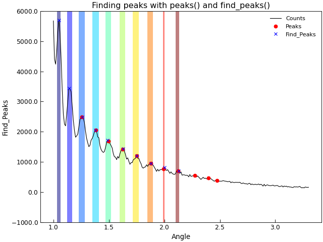
Peak Finding

Peak finding is a tricky and often required task in experimental data analysis. When a functional form is known, it is possible to fit the data to this functional form. However, often a more numerical approach is required. The AnalysisMixin.peaks() provides a relatively simple and effective method for doing this:

peak_data=peaks()
peak_data=peaks(ycol="Y Data", width=0.15, significance=0.001 , xcol="X Data", peaks=True, troughs=False, poly=2,  sort=True)

The xcol and ycol arguments index the columns with the relevant data. If xcol is not provided then the row number is used instead. If ycol is not provided then both x and y data is taken from the setas attribute.

The algorithm used is to differentiate the data with a Savitsky-Golay filter - which in effect fits a polynomial locally over the data. Zero crossing values in the derivative are located and then the second derivative is found for these points and are used to identify peaks and troughs in the data. The width and poly keywords are used to control the order of polynomial and the width of the window used for calculating the derivative - a lower order of polynomial and wider width will make the algroithm less sensitive to narrow peaks. The significance parameter controls which peaks and troughs are returned. If significance is a float, then only peaks and troughs whose second derivatives are larger than significance are returned. If significance is an integer, then maximum snd derivative in the data is divided by the supplied significance and used as the threshold on which peaks and troughs to return. If significance is not provided then a value of 20 is used. Finally, if sort is True, the peaks are returned in order of their significance. peaks and troughs select whether to return peaks or troughs.

The default values of width and saignificance are set on the assumption that a data set will have less than about 10 peaks of more or less equal significance. By default, only peaks are returned in order of x position.

The example below shows how to use AnalysisMixin.peaks() to filter out just the peak positions in a set of data.

"""Detect peaks in a dataset."""
from matplotlib.cm import jet
from numpy import linspace

from Stoner import Data

d = Data("../../sample-data/New-XRay-Data.dql")
e = d.clone
d.plot()
d.peaks(width=0.08, poly=4, significance=100, modify=True)
d.labels[1] = "Peaks"
d.plot(fmt="ro")
e.find_peaks(modify=True, prominence=80, width=0.01)
e.labels[1] = "Find_Peaks"
e.plot(figure=d.fig, fmt="bx")
d.title = "Finding peaks with peaks() and find_peaks()"

# Use the metadata that find_peaks produces
colors = jet(linspace(0, 1, len(e)), alpha=0.5)
for l, r, c in zip(e["left_ips"], e["right_ips"], colors):
    ax = d.axes[d.ax]
    ax.axvspan(l, r, facecolor=c)

(png, hires.png, pdf)