Data.scale
- Data.scale(other, xcol=None, ycol=None, xmode='linear', ymode='linear', use_estimate=False, bounds=None, otherbounds=None, replace=True, headers=None)
Scale the x and y data in this DataFile to match the x and y data in another DataFile.
- Parameters:
datafile (Data) – Data object to work with if not being used as a bound method.
other (DataFile) – The other instance of a datafile to match to
- Keyword Arguments:
xcol (column index) – Column with x points in it, default to None to use setas attribute value
ycol (column index) – Column with ypoints in it, default to None to use setas attribute value
xmode ('affine', 'linear','scale','offset') – How to manipulate the x-data to match up
ymode ('linear','scale','offset') – How to manipulate the y-data to match up.
bounds (callable) – Used to identiyf the set of (x,y) points to be used for scaling. Defaults to the whole data set if not speicifed.
otherbounds (callable) – Used to detemrine the set of (x,y) points in the other data file. Defaults to bounds if not given.
use_estimate (bool or 3x2 array) – Specifies whether to estimate an initial transformation value or to use the provided one, or start with an identity transformation.
replace (bool) – Whether to map the x,y data to the new coordinates and return a copy of this Stoner.Data (true) or to just return the results of the scaling.
headers (2-element list or tuple of strings) – new column headers to use if replace is True.
- Returns:
(various) – Either a copy of the :py:class:Stoner.Data` modified so that the x and y columns match other if replace is True, or opt_trans,*trans_err*,*new_xy_data*. Where opt_trans is the optimum affine transformation, trans_err is a matrix giving the standard error in the transformation matrix components and new_xy_data is an (n x 2) array of the transformed data.
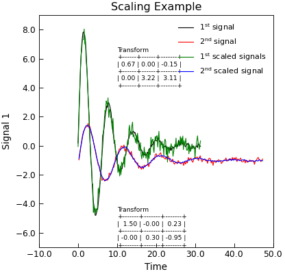
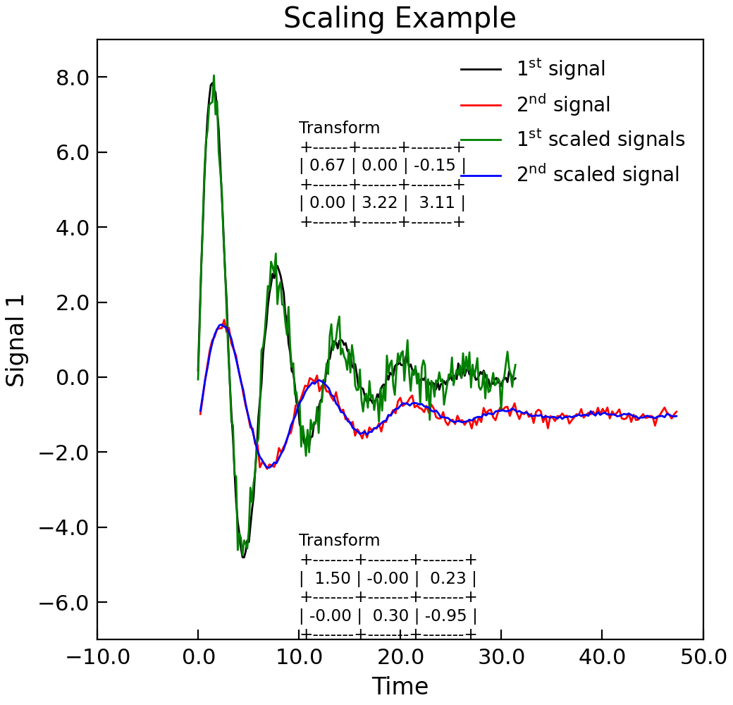
Example
"""Example of using scale to overlap data."""

import matplotlib as mpl
from numpy import column_stack, exp, linspace, pi, sin
from numpy.random import normal, seed
from tabulate import tabulate

from Stoner import Data

seed(3)  # Just fix the random numbers to stop optimizer warnings
mpl.rc("text", usetex=True)


x = linspace(0, 10 * pi, 201)
x2 = x * 1.5 + 0.23
y = 10 * exp(-x / (2 * pi)) * sin(x) + normal(size=len(x), scale=0.1)
y2 = 3 * exp(-x / (2 * pi)) * sin(x) - 1 + normal(size=len(x), scale=0.1)

d = Data(x, y, column_headers=["Time", "Signal 1"], setas="xy")
d2 = Data(x2, y2, column_headers=["Time", "Signal 2"], setas="xy")

d.plot(label="1$^\\mathrm{st}$ signal")
d2.plot(figure=d.fig, label="2$^\\mathrm{nd}$ signal")
d3 = d2.scale(d, headers="Signal 2 scaled", xmode="affine")
d3.plot(figure=d.fig, label="1$^\\mathrm{st}$ scaled signals")
d3["test"] = linspace(1, 10, 10)
txt = tabulate(d3["Transform"], floatfmt=".2f", tablefmt="grid")
d3.text(10, 4, f"Transform\n{txt}", fontdict={"size": "x-small"})

np_data = column_stack((x2, y2))
d4 = d.scale(
    np_data, headers="Signal 2 scaled", xmode="affine", use_estimate=True
)
d4.plot(figure=d.fig, label="2$^\\mathrm{nd}$ scaled signal")
d4.ylim = (-7, 9)
txt = tabulate(d4["Transform"], floatfmt=".2f", tablefmt="grid")
d4.text(10, -7, f"Transform\n{txt}", fontdict={"size": "x-small"})

d4.title = "Scaling Example"
