Curve Fitting in the Stoner Package

Introduction

Many data analysis tasks make use of curve fitting at some point - the process of fitting a model to as set of data points and determining the co-efficients of the model that give the best fit. Since this is such a ubiquitous task, it will be no surprise that the Stoner package provides a variety of different algorithms.

The choice of algorithm depends to a large part on the features of the model, the constraints on the problem and the nature of the data points to be fitted.

In order of increasing complexity, the Stoner package supports the following:

• Simple polynomial fits

  If the model is simply a polynomial function and there are no uncertainties in the data and no constraints on the parameters, then this is the simplest and easiest to use. This makes use of the Data.polyfit() method.

• Simple function fitting

  If you need to fit to an arbitrary function, have no constraints on the values of the fitting parameters, and have uncertainties in the y coordinates but not in the x, then the simple function fitting is probably the best option. The Stoner package provides a wrapper around the standard scipy.optimize.curve_fit() function in the form of the Data.curve_vit() method.

• Fitting with limits

  If your problem has constrained parameters - that is there are physical reasons why the parameters in your model cannot take certain values, the you probably want to use the Data.lmfit() method. This works well when your data has uncertainties in the y values but not in x.

• Orthogonal distance regression

  Finally, if your data has uncertainties in both x and y you may want to use the Data.odr() method to do an analysis that minimizes the distance of the model function in both x and y.

• Differential Evolution Algorithm

  Differential evolution algorithms attempt to find optimal fits by evaluating a population of possible solutions and then combining those that were scored by some costing function to be the best fits - thereby creating a new population of possible (hopefully better) solutions. In general some level of random fluctuation is permitted to stop the minimizer getting stuck in local minima. These algorithms can be effective when there are a karge number of parametgers to search or the cost is not a smooth function of the parameters and thus cannot be differentiated. The algorithm here uses a standard weighted variance as the cost function - like lmfit and curve_fit do.

Why Use the Stoner Package Fitting Wrappers?

There are a number of advantages to using the Stoner package wrappers around the the vartious fitting algorithms rather than using them as standalone fitting functions:

1. They provide a consistent way of defining the model to be fitted. All of the Stoner package functions accept a model function of the form: f(x,p1,p2,p3), constructing the necessary intrermediate model class as necessary - similatly they can all take an lmfit.model.Model class or instance and adapt that as necessary.

2. They provide a consistent parameter order and keyword argument names as far as possible within the limits of the underlying algorithms. Gerneally these follow the scipy.optimize.curve_fit() conventions.

3. They make use of the Data.setas attribute to identify data columns containing x, y and associated uncertainties. They also probvide a common way to select a subset of data to use for the fitting through the bounds keyword argument.

4. They provide a consistent way to add the best fit data as a column(s) to the Data object and to stpore the best-fit parameters in the metadata for retrieval later. Since this is done in a consistent fashion, the package also can probide a Data.annotate_plot() method to diisplay the fitting parameters on a plot of the data.

Simple polynomial Fits

Simple least squares fitting of polynomial functions is handled by the Data.polyfit() method:

a.polyfit(column_x,column_y,polynomial_order, bounds=lambda x, y:True,result="New Column")

This is a simple pass through to the numpy routine of the same name. The x and y columns are specified in the first two arguments using the usual index rules for the Stoner package. The routine will fit multiple columns if column_y is a list or slice. The polynomial_order parameter should be a simple integer greater or equal to 1 to define the degree of polynomial to fit. The bounds function follows the same rules as the bounds function in Data.search() to restrict the fitting to a limited range of rows. The method returns a list of coefficients with the highest power first. If column_y was a list, then a 2D array of coefficients is returned.

If result is specified then a new column with the header given by the result parameter will be created and the fitted polynomial evaluated at each point.

Fitting Arbitrary Functions

Common features of the Function Fitting Methods

he output of the three methods used to fit arbitrary functions depend on the keyword parameters output, result replace and header in the method call.

• output=”fit” The optimal parameters and a variance-covariance matrix are returned

• output=”row” A 1D numpy array of optimal values and standard errors interleaved (i.e. p_opt[0],p_error[0],p_opt[1],p_error[1]….) us returned. This is useful when analysing a large number of similar data sets in order to build a table of fitting results.

• output=”report” A python object representing the fitting reult is returned.

• output=”data” A copy for the data file itself is returned - this is most useful when used in conjunction with Stoner.DataFolder

• oputput=”full” As much information about the fit as can be extracted from the fitting algorithm is returned.

If result is not None, then the best fit data points are calculated and also the fitting parameters, errors and \(\chi^2\) value is calculated and added to the metadata of the Data object. To distinguish between multiple fits, a prefix keyword can be given, otherwise the default is to use a prefix derived from the name of the model that was fitted. result and replace control where the best fit datapoints are added to the Data obhject. If replace is True then it is added to the end of the Data object and replace is ignored. Otherwise, result is interpreted as something that can be used as a column index and replace determines whether the new data is inserted after that column, or overwrites it.

If residuals is not None or False then as well as calculating the best fit values, the difference between these and the data points is found. The value of residuals is either a column index to store the residuals at (or in if replace is True) or if True, then the column after the one specofied by result is used.

In all cases header specifies the name of the new header - if omitted, it will default to ‘Fitted with {model name}’.

The utility method of the Stoner.Core.Data, Stoner.Util.Data.annotate_fit() is useful for adding appropriately formatted details of the fit to the plot (in this case for the case of Simple function fitting).

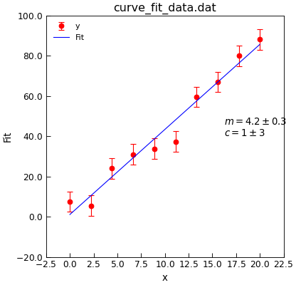
"""USe curve_fit to fit a straight line."""
from Stoner import Data


def linear(x, m, c):
    """Straight line function."""
    return m * x + c


d = Data("curve_fit_data.dat", setas="xye")
d.plot(fmt="ro")
fit = d.curve_fit(
    linear, result=True, replace=False, header="Fit", output="report"
)
d.setas = "x..y"
d.plot(fmt="b-")
d.annotate_fit(linear)
d.draw()
print(fit.fit_report())

(png, hires.png, pdf)

The bounds function can be used to restrict the fitting to only a subset of the rows of data. Any callable object which will take a float and an array of floats, representing the one x-value and one complete row and return True if the row is to be included in the fit and False if not. e.g.:

def bounds_func(x,row):
"""Keep only data points between (100,5) and (200,20) in x and y.

x (float): x data value
row (DataArray): complete row of data."""
    return 100<x<200 and 5<row.y<20

Simple function fitting

For more general curve fitting operations the Data.curve_fit() method can be employed. Again, this is a pass through to the numpy routine of the same name.:

a.curve_fit(func,  xcol, ycol, p0=None, sigma=None,[absolute_sigma=True|scale_covar=False], bounds=lambda x, y: True,
    result=True,replace=False,header="New Column" )

The first parameter is the fitting function. This should have prototype y=func(x,p[0],p[1],p[2]...): where p is a list of fitting parameters.

Alternatively a subclass of, or instance of, a lmfit.model.Model can also be passed and it’s function will be used to provide information to Data.curve_fit().

The p0 parameter contains the initial guesses at the fitting parameters, the default value is 1. xcol and ycol are the x and y columns to fit. If xcol and ycol are not given, then the Data.setas attrobite is used to determine which columns to fit.

sigma, absolute_sigma and scale_covar determine how the fitting process takes account of uncertainties in the y data. sigma, if present, provides the weightings or standard deviations for each datapoint and so should also be an array of the same length as the x and y data. If sigma is not given and a column is identified int he Data.setas attribute as containing e values, then that is used instead. If absolute_sigma is given then if this is True, the sigma values are interpreted as absolute uncertainties in the data points, if it is False, then they are relative weightings. If absolute_sigma is not given, a scale_covar parameter will have the same effect, but inverted, so that True equates to relative weights and False to absolute uncertainties. Finally if neither is given then any sigma values are assumed to be absolute.

If a variance-co-variance matrix is returned frpom the fit then this can be used to calculate the estimated standard errors in the fitting parameters:

p_error=np.sqrt(np.diag(p_cov))

THe off-diagonal terms of the variance-co-variance matrix give the co-variance between the fitting parameters. LArge absolute values of these terms indicate that the parameters are not properly independent in the model.

Fitting with limits

The Stoner package has a number of alternative fitting mechanisms that supplement the standard scipy.optimize.curve_fit() function. New in version 0.2 onwards of the Package is an interface to the lmfit module.

lmfit provides a flexible way to fit complex models to experimental data in a pythonesque object-orientated fashion. A full description of the lmfit module is given in the lmffit documentation. . The Data.lmfit() method is used to interact with lmfit.

In order to use Data.lmfit(), one requires a lmfit.model.Model instance. This describes a function and its independent and fittable parameters, whether they have limits and what the limits are. The Stoner.Fit module contains a series of lmfit.model.Model subclasses that represent various models used in condensed matter physics.

The operation of Data.lmfit() is very similar to that of Data.curve_fit():

from Stoner.analysis.fitting.models.thermal import Arrehenius
model=Arrehenius(A=1E7,DE=0.01)
fit=a.lmfit(model,xcol="Temp",ycol="Cond",result=True,header="Fit")
print fit.fit_report()
print a["Arrehenius:A"],a["Arrehenius:A err"],a["chi^2"],a["nfev"]

In this example we would be fitting an Arrehenius model to data contained in the ‘Temp’ and ‘Cond’ columns. The resulting fit would be added as an additional column called fit. In addition, details of the fit are added as metadata to the current Data.

The model argument to Data.lmfit() can be either an instance of the model class, or just the class itself (in which case it will be instantiated as required), or just a bare callable, in which case a model class will be created around it. The latter is approximately equivalent to a simple call to Data.curve_fit().

The return value from Data.lmfit() is controlled by the output keyword parameter. By default it is the lmfit.model.ModelFit instance. This contains all the information about the fit and fitting process.

You can pass the model as a subclass of model, if you don’t pass initial values either via the p0 parameter or as keyword arguments, then the model’s guess method is called (e.g. Stoner.analysis.fitting.models.thermal.Arrhenius.guess()) to determine parameters fromt he data. For example:

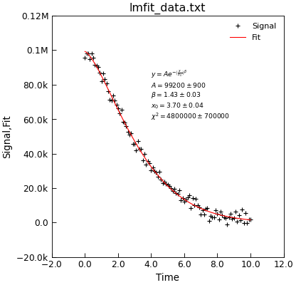
"""Example of using lmfit to do a bounded fit."""
from Stoner import Data
from Stoner.analysis.fitting.models.generic import StretchedExp

# Load dat and plot
d = Data("lmfit_data.txt", setas="xy")
d.y = d.y

# Do the fit
d.lmfit(StretchedExp, result=True, header="Fit", residuals=True)
# plot
d.setas = "xyy"

d.plot(fmt=["+", "-"])
# Make apretty label using Stoner.Util methods
text = r"$y=A e^{-\left(\frac{x}{x_0}\right)^\beta}$" + "\n"
text += d.annotate_fit(StretchedExp, text_only=True)
d.text(4, 6e4, text, fontsize="x-small")

(png, hires.png, pdf)

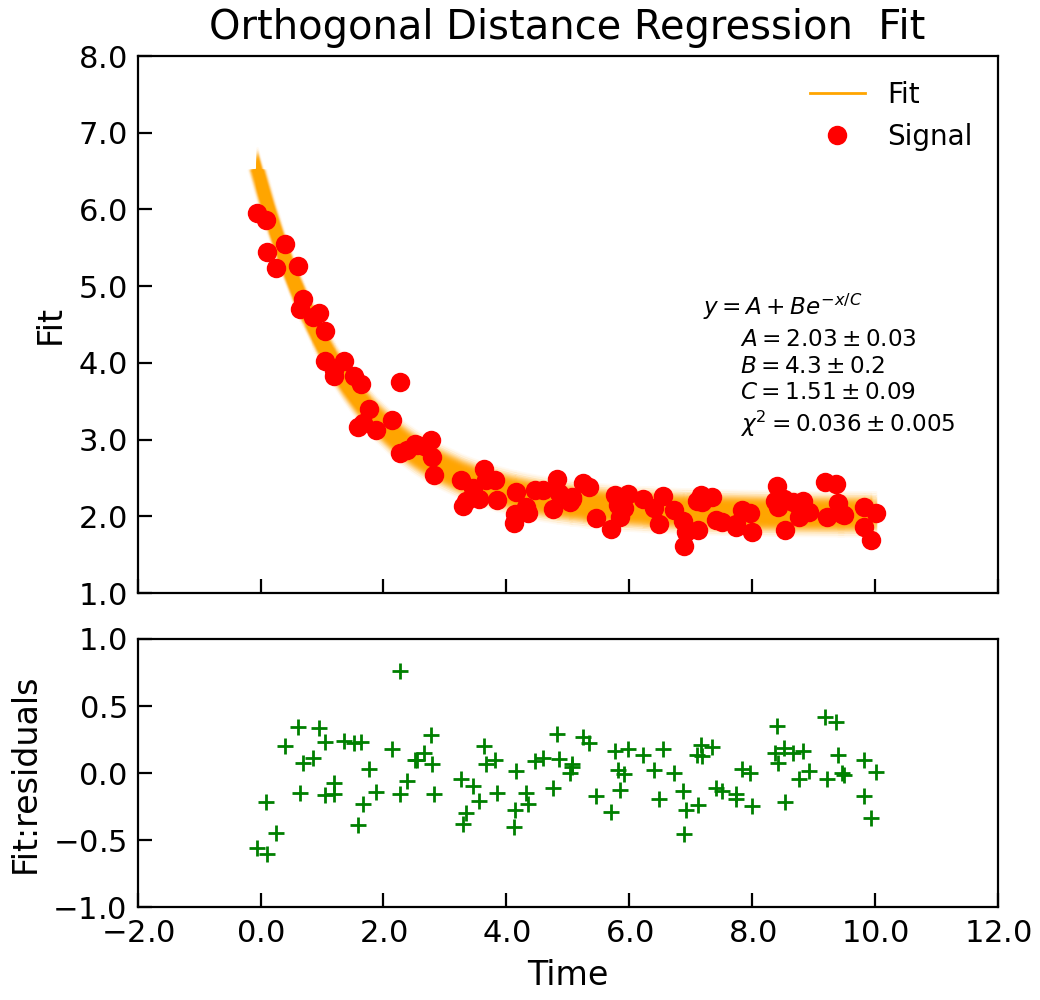
Orthogonal distance regression

Data.curve_fit() and Data.lmfit() are both essentially based on a Levenberg-Marquardt fitting algorithm which is a non-linear least squares routine. The essential point is that it seeks to minimize the vertical distance between the model and the data points, taking into account the uncertainty in the vertical position (ie. y coordinate) only. If your data has peaks that may change position and/or uncertanities in the horizontal (x) position of the data points, you may be better off using an orthogonal distance regression.

The Data.odr() method wraps the scipy.odr module and tries to make it function as much like lmfit as possible. In fact, in most cases it can be used as a drop-in replacement:

"""Simple use of lmfit to fit data."""
from numpy import linspace, exp, random

from Stoner import Data
from Stoner.plot.utils import errorfill

random.seed(12345)  # Ensure consistent random numbers!

# Make some data
x = linspace(0, 10.0, 101)
y = 2 + 4 * exp(-x / 1.7) + random.normal(scale=0.2, size=101)
x += +random.normal(scale=0.1, size=101)

d = Data(x, y, column_headers=["Time", "Signal"], setas="xy")

func = lambda x, A, B, C: A + B * exp(-x / C)

# Do the fitting and plot the result
fit = d.odr(
    func,
    result=True,
    header="Fit",
    A=1,
    B=1,
    C=1,
    prefix="Model",
    residuals=True,
)

# Reset labels
d.labels = []

# Make nice two panel plot layout
ax = d.subplot2grid((3, 1), (2, 0))
d.setas = "x..y"
d.plot(fmt="g+")
d.title = ""

# Plot up the data
ax = d.subplot2grid((3, 1), (0, 0), rowspan=2)
d.setas = "xy"
d.plot(fmt="ro")

d.setas = "x.y"
d.plot(plotter=errorfill, yerr=0.2, color="orange")
d.plot(plotter=errorfill, xerr=0.1, color="orange", label=None)
d.xticklabels = [[]]
d.xlabel = ""

# Annotate plot with fitting parameters
d.annotate_fit(func, prefix="Model", x=0.7, y=0.3, fontdict={"size": "x-small"})
text = r"$y=A+Be^{-x/C}$" + "\n\n"
d.text(7.2, 3.9, text, fontdict={"size": "x-small"})
d.title = "Orthogonal Distance Regression  Fit"

(png, hires.png, pdf)

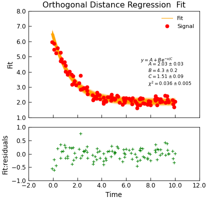
The Data.odr() method allows uncertainties in x and y to be specified via the sigma_x and sigma_y parameters. If either are not specified, and a sigma parameter is given, then that is used instead. If they are either explicitly set to None or not given, then the Data.setas attribute is used instead.

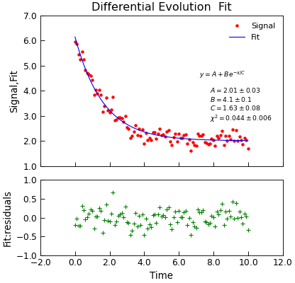
Differential Evolution Algorithm

When the number of parameters gets large it can get increasingly difficult to get fits using the techniques above. In these situations, the differential evolution approach may be valuable. The Stoner.Data.differential_evolution() method provides a wrapper around the scipi.optimize.differential_evolution() minimizer with the advantage that the model specification, and calling signatures are essentially the same as for the other fitting functions and thus there is little programmer overhead to switching to it:

"""Simple use of lmfit to fit data."""
from numpy import linspace, exp, random

from Stoner import Data

random.seed(12345)  # Ensure consistent random numbers!
# Make some data
x = linspace(0, 10.0, 101)
y = 2 + 4 * exp(-x / 1.7) + random.normal(scale=0.2, size=101)

d = Data(x, y, column_headers=["Time", "Signal"], setas="xy")

func = lambda x, A, B, C: A + B * exp(-x / C)


# Do the fitting and plot the result
fit = d.differential_evolution(
    func,
    result=True,
    header="Fit",
    A=1,
    B=1,
    C=1,
    prefix="Model",
    residuals=True,
)

# Reset labels
d.labels = []

# Make nice two panel plot layout
ax = d.subplot2grid((3, 1), (2, 0))
d.setas = "x..y"
d.plot(fmt="g+")
d.title = ""

ax = d.subplot2grid((3, 1), (0, 0), rowspan=2)
d.setas = "xyy"
d.plot(fmt=["r.", "b-"])
d.xticklabels = [[]]
d.xlabel = ""

# Annotate plot with fitting parameters
d.annotate_fit(func, prefix="Model", x=0.7, y=0.3, fontdict={"size": "x-small"})
text = r"$y=A+Be^{-x/C}$" + "\n\n"
d.text(7.2, 3.9, text, fontdict={"size": "x-small"})
d.title = "Differential Evolution  Fit"

(png, hires.png, pdf)

Intrinsically, the differential evolution algorithm does not calculate a variance-covariance matrix since it never needs to find the gradient of the \(\chi^2\) of the fit with the parameters. In order to provide such an estimate, the Stroner.Data.differential_evolution() method carries out a standard least-squares non-linear fit (using scipy.optimize.curve_fit()) as a second stage once scipy.optimize.differential_evolution() has foind a likely goot fitting set of parameters. This hybrid approach allows a good fit location to be identified, but also the physically useful fitting errors to be estimated.

Included Fitting Models

The Stoner.analysis.fitting.models module provides a number of standard fitting models suitable for solida state physics. Each model is provided either as an lmfit.model.Model and callable function. The former case often also provides a means to guess initial values from the data.

Elementary Models

Amongst the included models are very generic model functions (in Stoner.analysis.fitting.models.generic) including: .. currentmodule:: Stoner.analysis.fitting.models.generic

• Linear - straight line fit \(y=mx+c\)

• Quadratic - 2nd order polynomial \(y=ax^2+bx+c\)

• PowerLaw - A general powerlaw expression \(y=Ax^k\)

• StretchedExponential is a standard exponential decay with an additional power \(\beta\) - \(y=A\exp\left[\left(\frac{-x}{x_0}\right)^\beta\right]\)

Thermal Physics Models

The Stoner.analysis.fitting.models.thermal module supports a range of models suitable for various thermal physics related expressions: .. currentmodule:: Stoner.analysis.fitting.models.thermal

• Arrhenius - The Arrhenius expression is used to describe processes whose rate is controlled by a thermal distribution, it is essentially an exponential decay \(y=A\exp\left(\frac{-\Delta E}{k_Bx}\right)\).

• ModArrhenius - The modified Arrhenous expresses \(\tau=Ax^n\exp\left(\frac{-\Delta E}{k_B x}\right)\) is used when the prefactor in the regular Arrhenius theory has a temperature dependence. Typically the prefactor exponent ranges for \(-1<n<1\).

• NDimArrhenius is suitable for thermally activated transport in more than 1 dimension, or in variable range hopping processes - \(\tau=A\exp\left(\frac{-\Delta E}{k_B x^n}\right)\)

• VFTEquation - the Vogel-Flucher-Tammann Equation is another modification of the Arrhenius equiation which can apply when a process has both an activation energy and a threshold temperature (duue to a phase transition for example) and is given by \(\tau = A\exp\left(\frac{\Delta E}{x-x_0}\right)\)

Tunnelling Electron Transport Models

We also have a number of models for electron tunnelling processes built into the library in Stoner.analysis.fitting.models.tunnelling: .. currentmodule:: Stoner.analysis.fitting.models.tunnelling

• Simmons - the Simmons model describes tunneling through a square barrer potential for the limit where the barrier height is comparable to the junction bias.

• BDR - this model introduces a trapezoidal barrier where the barrier height is different between the two electrondes - e.g. where the electrodes are composed of different materials.

• FowlerNordheim - this is another simplified model of electron tunneling that has a single barrier height and width parameters.

• Stoner.Fit.TersoffHammann - this model just treats tunneling as a linear I-V process and is applicable when the barrier height is large compared to the bias across the tunnel barrier.

Magnetism Related Models

The Stoner.analysis.fitting.models.magnetism includes models related to magnetism and magnetic materials. .. currentmodule:: Stoner.analysis.fitting.models.magnetism

• Langevin model is used to describe the magnetic moment versus field of a paramagnet.

• KittelEquation and Stoner.Fit.Inverse_Kittel - the Kittel equation is used to described the magnetic field and frequency response of the ferromagnetic resonance peak.

• KittelEquation and Inverse_Kittel - the Kittel equation is used to described the magnetic field and frequency response of the ferromagnetic resonance peak.

Peak Models

The lmfit package comes with several common peak function models built in which can be used firectly. The Stoner package adds a coouple more to the selection - these are particularly useful for fitting ferromagnetic resonance data:

• Lorentzian_diff - the lmfit module includes built in classes for Lorentzian peaks - but this model is the differential of a Lorentzian peak.

• FMR_Power - although this model is usually used specifically for calculating the absorption spectrum for a Ferromagnetic Resonance process, it is in fact a generic combination of both Lorentzian peak and differential forms.

Superconductivity Related Models

The Stoner.analysis.fitting.models.superconductivity offers some models related to superconducting materials and devices. .. currentmodule:: Stoner.analysis.fitting.models.superconductivity

• Strijkers - this tunnel model describes electrons passing from a superconductor to a non-superconductor with a potential step or barrier between the two. In one limit it describes Andreev reflection in a clean interface and in the other, a Giaever Junction (S-I-N).

Other Electrical Transport Models

Finally we incliudde some other common electrical transport models for solid-state physics in the Stoner.analysis.fitting.models.e_transport module. .. currentmodule:: Stoner.analysis.fitting.models.e_transport

• BlochGrueneisen - this model describes electrical resistivity of a metal as a function of temperature and can be used to extract the Debye temperature \(\Theta_D\).

• FluchsSondheimer - this model describes the electrical resistivity of a thin film as a function of its thickness and can be used to extract a mean free path :math: lambda_{mfp} and intrinsic conductivity.

• WLfit - the weak localisation fit can be used to describe rthe magnetoconductance of a system with sufficient scattering that weak-localisation effects appear,

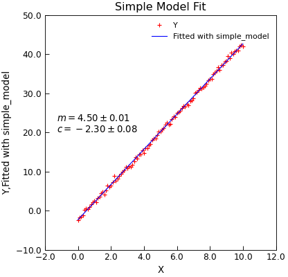
Making Fitting Models

You can simply pass a bare function to any of the general fitting meothods, but there can be advantages in using an lmfit.Model class - such as the ability to combine several models together, the ability to guess parameters or just for the readability. The Stoner package provides some tools to help make suitable model classes.

Stoner.Fit.make_model() is a python decorator function that can do the leg-work of transforming a simple model function of the form:

@make_model
def model_func(x_data,param1,param2):
    return f(x,param1,param2)

into a suitable model class of the same name. This model class then provides a decorator function itself to mark a second function as something that can be used to guess parameter values:

@model_func.guesser
def model_guess(y_data,x=x_data):
    return [param1_guess,param2_guess]

In the same vein, the class provides a decorator to use a function to generate hints about the parameter, such as bounding values:

@model_func.hinter
def model_parameter_hints():
    return {"param1":{"max":10.0, "min":1.0},"param2":{"max":0.0}}

the newly created model_func class can then be used immediately to fit data. The following example illustrates the concept.

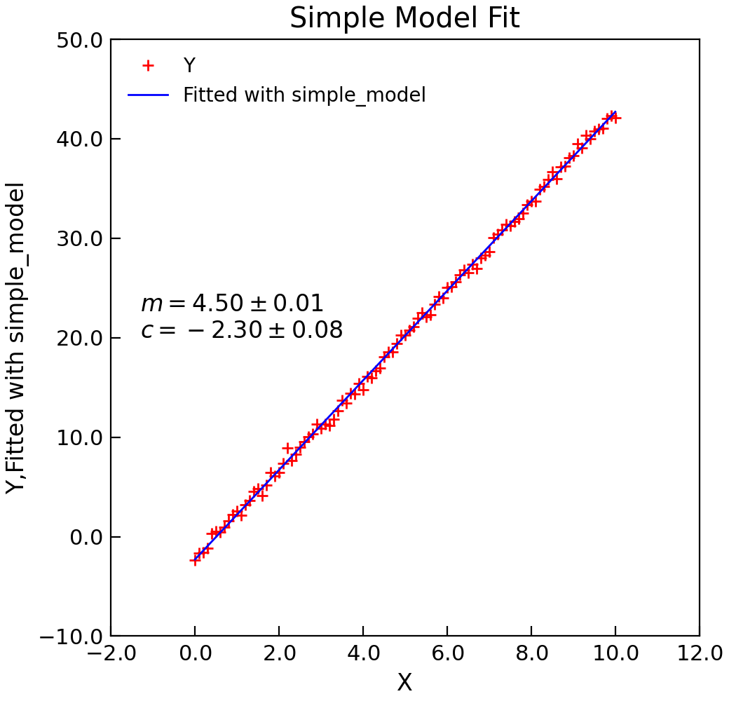
#!/usr/bin/env python3
# -*- coding: utf-8 -*-
"""Demo of the make_model decorator."""
from numpy import linspace
from numpy.random import normal, seed

from Stoner import Data
from Stoner.analysis.fitting.models import make_model

seed(12345)  # Ensure consistent random numbers


# Make our model
@make_model
def simple_model(x, m, c):
    """A straight line."""
    return x * m + c


# Add a function to guess parameters (optional, but)
@simple_model.guesser
def guess_vals(y, x=None):
    """Should guess parameter values really!"""
    m = (y.max() - y.min()) / (x[y.argmax()] - x[y.argmin()])
    c = x.mean() * m - y.mean()  # return one value per parameter
    return [m, c]


# Add a function to sry vonstraints on parameters (optional)
@simple_model.hinter
def hint_parameters():
    """Five some hints about the parameter."""
    return {"m": {"max": 10.0, "min": 0.0}, "c": {"max": 5.0, "min": -5.0}}


# Create some x,y data
x = linspace(0, 10, 101)
y = 4.5 * x - 2.3 + normal(scale=0.4, size=len(x))

# Make The Data object
d = Data(x, y, setas="xy", column_headers=["X", "Y"])

# Do the fit
d.lmfit(simple_model, result=True)

# Plot the result
d.setas = "xyy"
d.plot(fmt=["r+", "b-"])
d.title = "Simple Model Fit"
d.annotate_fit(simple_model, x=0.05, y=0.5)

(png, hires.png, pdf)

Advanced Fitting Topics

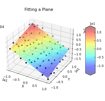
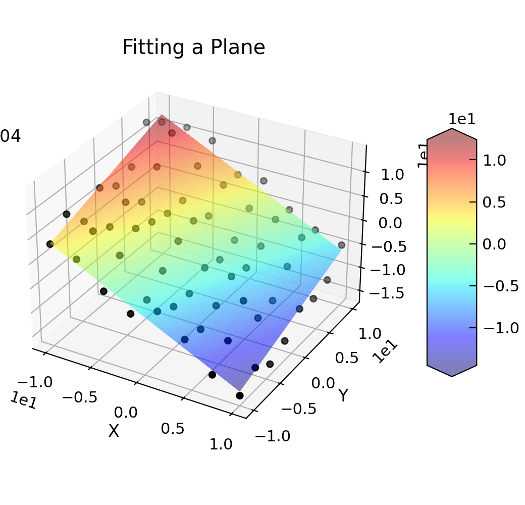
Fitting In More than 1D

Data.curve_fit() can also be used to fit more complex problems. In the example below, a set of points in x,y,z space are fitted to a plane.

"""Use curve_fit to fit a plane to some data."""
from numpy.random import normal, seed
from numpy import linspace, meshgrid, column_stack, array
import matplotlib.cm as cmap

from Stoner import Data

seed(12345)  # Ensire consistent random numbers!


def plane(coord, a, b, c):
    """Function to define a plane."""
    x, y = coord.T
    return c - (x * a + y * b)


coeefs = [1, -0.5, -1]
col = linspace(-10, 10, 8)
X, Y = meshgrid(col, col)
Z = plane(array([X, Y]).T, *coeefs) + normal(size=X.shape, scale=2.0)
d = Data(
    column_stack((X.ravel(), Y.ravel(), Z.ravel())),
    filename="Fitting a Plane",
    setas="xyz",
)

d.column_headers = ["X", "Y", "Z"]
d.plot_xyz(plotter="scatter", title=None, griddata=False, color="k")

popt, pcov = d.curve_fit(plane, [0, 1], 2, result=True)
col = linspace(-10, 10, 128)
X, Y = meshgrid(col, col)
Z = plane(array([X, Y]).T, *popt)
e = Data(
    column_stack((X.ravel(), Y.ravel(), Z.ravel())),
    filename="Fitting a Plane",
    setas="xyz",
)
e.column_headers = d.column_headers

e.plot_xyz(linewidth=0, cmap=cmap.jet, alpha=0.5, figure=d.fig)

txt = "$z=c-ax+by$\n"
txt += "\n".join(
    [d.format("plane:{}".format(k), latex=True) for k in ["a", "b", "c"]]
)

ax = d.axes[0]
ax.text(-30, -10, 10, txt)

(png, hires.png, pdf)

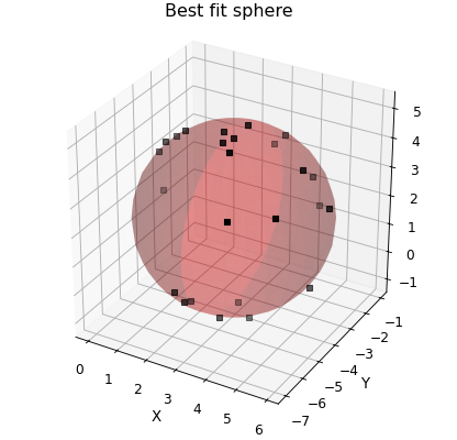
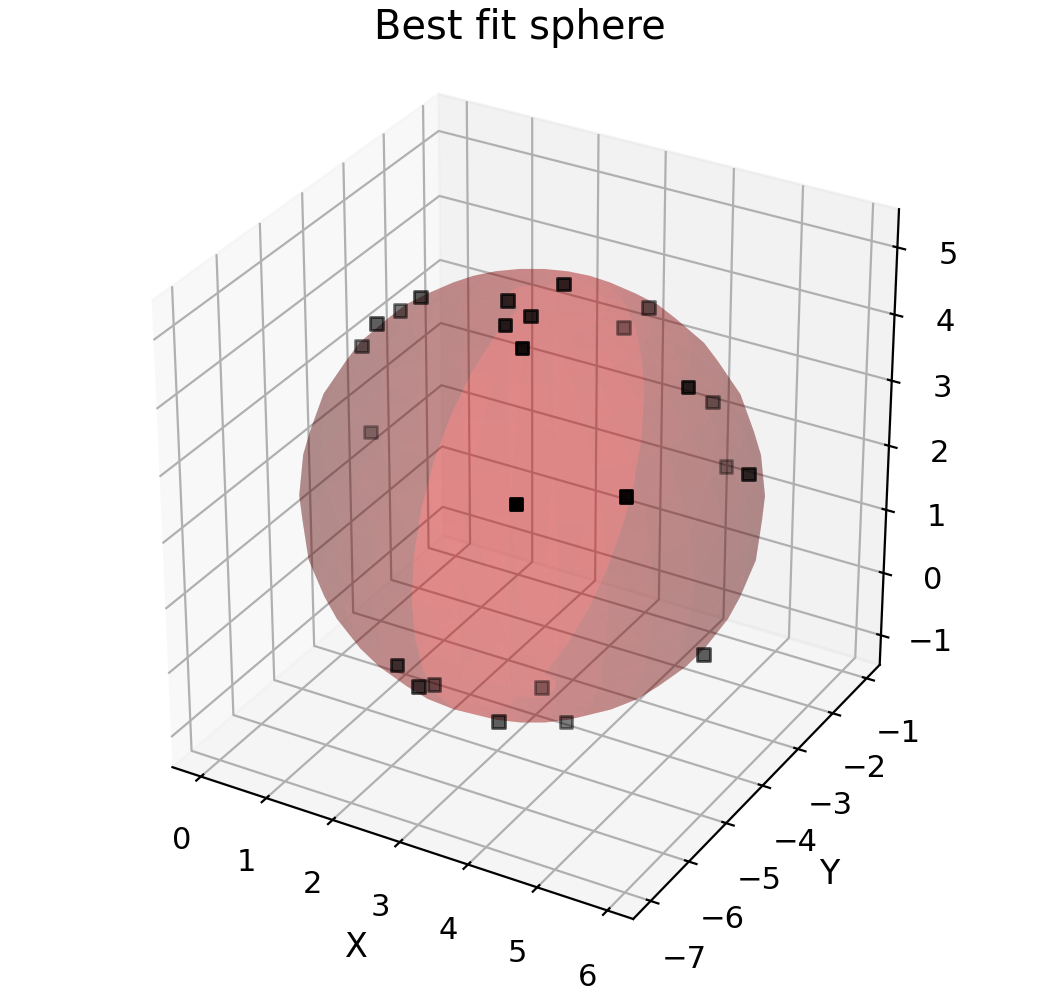
Finally, by you can specify the y-data to fit to as a numpy array. This can be used to fit functions that don’t themseleves return values that can be matched up to existing data. An example of doing this is fitting a sphere to a set of \((x,y,z)\) data points. In this case the fitting parameters are \((x_0,y_0,z_0)\) for the centre of the sphere, \(r\) for the radius and the fitting equation is \((x-x_0)^2+(y-y_0)^2+(z-z_0)^2-r^2=0\) and so we pass an array of zeros as the y-data.

"""Fit a sphere with curve_fit."""
from numpy import (
    sin,
    cos,
    pi,
    column_stack,
    zeros_like,
    ones_like,
    meshgrid,
    linspace,
)
from numpy.random import normal, uniform, seed
import matplotlib.pyplot as plt

from Stoner import Data

seed(12345)  # Ensure consistent random numbers!


def transform(r, q, p):
    """Converts from spherical to cartesian coordinates."""
    x = r * cos(q) * cos(p)
    y = r * cos(q) * sin(p)
    z = r * sin(q)
    return x, y, z


def sphere(coords, a, b, c, r):
    """Returns zero if (x,y,z) lies on a sphere centred at (a,b,c) with radius r."""
    x, y, z = coords.T
    return (x - a) ** 2 + (y - b) ** 2 + (z - c) ** 2 - r**2


# Create some points approximately spherical distribution
num = 25
q = uniform(low=-pi / 2, high=pi / 2, size=num)
p = uniform(low=0, high=2 * pi, size=num)
r = normal(loc=3.0, size=num, scale=0.1)

x, y, z = transform(r, q, p)

x += 3.0
y -= 4.0
z += 2.0

# Construct the  DataFile object
d = Data(
    column_stack((x, y, z)),
    setas="xyz",
    filename="Best fit sphere",
    column_headers=["X", "Y", "Z"],
)
d.template.fig_width = 5.2
d.template.fig_height = 5.0  # Square aspect ratio
d.plot_xyz(plotter="scatter", marker=",", griddata=False)
d.set_box_aspect((1, 1, 1.0))  # Passing through to the current axes
# curve_fit does the hard work
popt, pcov = d.curve_fit(sphere, (0, 1, 2), zeros_like(d.x))

# This manually constructs the best fit sphere
a, b, c, r = popt
p = linspace(-pi / 2, pi / 2, 16)
q = linspace(-pi, pi, 31)
P, Q = meshgrid(p, q)
R = ones_like(P) * r
x, y, z = transform(R, Q, P)
x += a
y += b
z += c

ax = d.axes[0]
ax.plot_surface(
    x, y, z, rstride=1, cstride=1, color=(1.0, 0.0, 0.0, 0.25), linewidth=0
)
plt.draw()

(png, hires.png, pdf)

See also Fitting Tricks

Non-linear curve fitting with initialisation file

For writing general purpose fitting codes, it can be useful to drive the fitting code from a separate initialisation file so that users do not have to edit the source code. Data.lmfit() and Data.odr() combined with Stoner.Fit provide some mechanisms to enable this.

Firstly, the initialisation file should take the form like so.

[Options]
model: Stoner.analysis.fitting.models.superconductivity.Strijkers
# Controls whether the data and fit are plotted or not.
show_plot: True
# Sets whether to print a nice report to the console
print_report: True
# Save the final result ?
save_fit: False
#
# These are optional options that turn on various (experimental) bits of code
#
#This turns on the normalisation
normalise: False
# This turns on the fitting a quadratic to the outer 10% to determine the normalisation
# Don't use it unless you know why this might be sensible for your data !
fancy_normaliser: False
# Turns on rescaling the V axis into mV
# Only use if data not already correctly scaled.
rescale_v: False
# Tries to find and remove an offset in V by looking for peaks within 5 Delta
# Warning, this may go badly wrong with certain DC waveforms
remove_offset: False
# Decompose the data into symmetric and anti-symmetric with respect to bias and then fit the symmetric part only.
make_symmetric: True
# Be clever about annotating the result on the plots
fancy_result: True
#
# Can switch between a least-squares fitting algorithm based on the lmfit module, or othogonal distance regression "odr"
method=lmfit

# These settings will read old style files directly
[Data]
x: V
y: G
# This will load from a csv file, comment out to have it guess the file type
type: Stoner.formats.generic.CSVFile
header_line:1
start_line:2
separator: ,
# Only need v_scale if rescale_v is true
v_scale:1000
# Only need this if normalise is True and fancy_normaliser is False
Normal_conductance: 0.0
# Set true to discard data at high bias
discard: False
# Bias limit to discard at
v_limit: 10.0


# The next four sections set the parameters up
[omega]
#starting value
value:0.55
# Allow this parameter to vary in the fix
vary: True
#Lower bound is set
min: 0.0
# Would give upper limit if it were constrained
# Just comment out limits which are not set
#max: None
# Symbol for plot annotations
label: \omega
# Default step size 0 . Use in conjunction with vary,min and max when mapping a parameter
step: 0.0
# Defines the units label for the plots
units: meV

[delta]
value: 1.5
vary: True
min: 0.5
max: 2.0
label: \Delta
step: 0.2
units: meV

[P]
value: 0.5
vary: True
min: 0.2
max: 0.7
label: P
step: 0.05

[Z]
value: 0.17
vary: True
min: 0.0
#max: None
label: Z
step: 0.0

This initialisation file can be passed to Stoner.Fit.cfg_data_from_ini() which will use the information in the [Data] section to read in the data file and identify the x and y columns.

The initialisation file can then be passed to Stoner.Fit.cfg_model_from_ini() which will use the configuration file to setup the model and parameter hints. The configuration file should have one section for eac parameter in the model. This function returns the configured model and also a 2D array of values to feed as the starting values to Data.lmfit(). Depending on the presence and values of the vary and step keys, tnhe code will either perform a single fitting attempt, or do a mapping of the \(\\chi^2\) goodeness of fit.

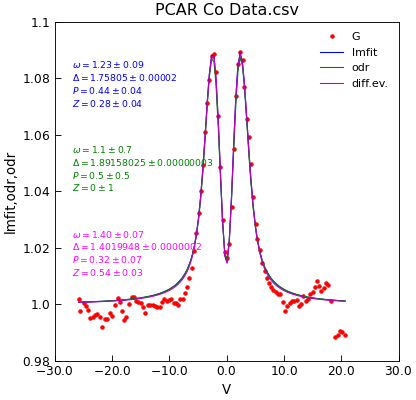
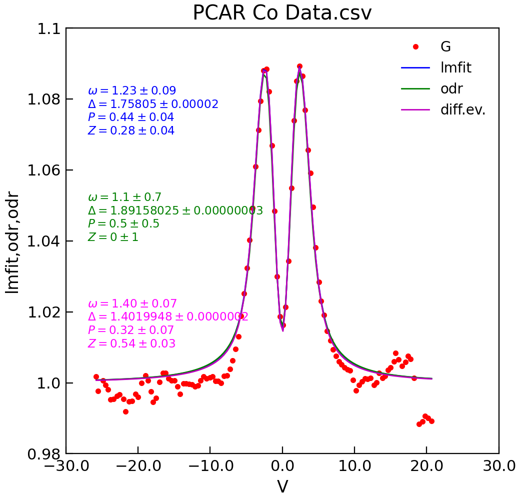
Since both the Data.odr() and Data.differential_evolution() supports the same interface, either can be used as a drop-in replacement as well. (Although it is interesting to note that in this example, they give quite different results - a matter of interest for the physics!)

"""Demo of new Stoner.Analysis.AnalyseFile.lmfit."""
from os.path import join

from Stoner.analysis.fitting.models import cfg_data_from_ini, cfg_model_from_ini
from Stoner import __home__

config = join(__home__, "..", "scripts", "PCAR-New.ini")
datafile = join(__home__, "..", "sample-data", "PCAR Co Data.csv")

d = cfg_data_from_ini(config, datafile)
model, p0 = cfg_model_from_ini(config, data=d)

d.x += 0.25
d.setas = "xy"
d.plot(fmt="r.")  # plot the data
fit = d.lmfit(model, result=True, header="lmfit")
fit = d.odr(model, result=True, header="odr", prefix="odr")
fit = d.differential_evolution(model, result=True, header="odr", prefix="diff")
d.setas = "x.yyy"
d.plot(fmt=["b-", "g-", "m-"], label=["lmfit", "odr", "diff.ev."])

d.annotate_fit(
    model, x=0.05, y=0.75, fontdict={"size": "x-small", "color": "blue"}
)
d.annotate_fit(
    model,
    x=0.05,
    y=0.5,
    fontdict={"size": "x-small", "color": "green"},
    prefix="odr",
)
d.annotate_fit(
    model,
    x=0.05,
    y=0.25,
    fontdict={"size": "x-small", "color": "magenta"},
    prefix="diff",
)

(png, hires.png, pdf)